In which we try to figure out what what’s going on with double-factorials.

This was formerly part of the previous post about \(n\)-spheres, but I started adding things to it and decided to split them up. It is not necessary to read the original previous post first, but this does sort of function as a sequel to it since it’s the direction my investigation has gone. Both articles are essentially unwieldy dumps for notes and calculations that I’ve done and make a record of. But maybe they’ll be useful as a survey of various related ideas, if anyone else is curious about this and comes across them.

My main finding is that I now believe we should be thinking of factorials as multiplicative integrals, like this:

\[\frac{n!}{m!} = \prod_m^n d^{\times}(x!)\]

And in particular, the factorials we’re used to have an implicit lower bound on that integral: the value \(n!\) is really \(\frac{n!}{0!} = \prod_0^n d^{\times}(x!)\). This means we never really “see the value” of \(0!\), because \(0!\) is equivalent to \(0!/0! = 1\). This interpretation seems to remove a bunch of ambiguity in the various definitions/analytic continuations of factorials on non-integer numbers (as well as explaining why those definitions don’t mess up the usual combinatoric sense of factorials).

Among other things, we find that the double-factorial function’s annoying asymptotic properties are entirely due to the fact that, for odd numbers, the integral stops at \(1\) instead of \(0\), so one piece is missing:

\[\prod_0^1 d^{\times}(n!!) = \sqrt{2} \prod_0^{1/2} d^{\times}(n!) = \sqrt{2} (\frac{1}{2})!= \sqrt{\frac{\pi}{2}}\]

Other than that, \(n!!\) is just a rescaled version of \(n!\):

\[n!! =2^{n/2} n! \times (\sqrt{\frac{\pi}{2}})^{n \text{ odd}}\]

Of course, factorials aren’t really integrals over continuous ranges, because they’re only defined on positive integers, so this is all hand-waving. We can’t claim to really know what the integrand \(d^{\times}(n!)\) actually “is” at a sub-integer level: \(\Gamma(n+1)\) is one interpolation that has some nice properties, but there is still something arbitrary about it, so we shouldn’t get too sure of ourselves; when we say that \((\frac{1}{2})! = \frac{\sqrt{\pi}}{2}\), we’re really claiming something about our favorite choice of interpolation for \(n!\), not about \(n!\) itself. There are good reasons for it, but it is still a choice until we have an argument otherwise. More on that towards the end, and maybe more in the future.

---

1. Investigations into double factorials

First we will study the double factorial function a bit and see how it interacts with half-integer single-factorials.

We’ll need some Gamma function/factorial identities for integer and half-integer values to start unpacking things. I don’t care much for the ways that everyone else writes them so here are my preferred versions.

The first few half-integer terms of \(\Gamma(x+1)\)/\(x!\) are:

\[\gdef\arraystretch{1.5} \begin{array}{rcccl} (-1/2)! &=& \Gamma(1/2) &=& \sqrt{\pi} \\ (1/2)! &=& \Gamma(3/2) &=& (\frac{1}{2}) \sqrt{\pi} \\ (3/2)! &=& \Gamma(5/2) &=& (\frac{3}{2}) (\frac{1}{2}) \sqrt{\pi} \end{array}\]

All of the structure here arises from \((-1/2)! = \sqrt{\pi}\): since \(n! = n (n-1)!\) continues to hold for non-integers you just find that \((5/2)! = 5/2 \times 3/2 \times 1/2 \times (-1/2)!\).

The value of \((-1/2)!\) seems essentially connected to the Gaussian integral \(\int_{-\infty}^{\infty} e^{-x^2} \d x = \sqrt{\pi}\); more on that another time. For now we take it as a given. Incidentally, other non-half-integer fractions of \(\Gamma\) also take values that sometimes have legible expressions (see here; for instance \(\Gamma(\frac{1}{4})\) is connected to the Leminscate in a manner similar to how \(\Gamma(\frac{1}{2})\) is connected to spheres)… but they are much harder to compute or make sense of.

(After this, I am going to not use the symbol \(\Gamma\) very much, except for connecting things to existing formulae. I prefer to write \(n!\) for \(\Gamma(n+1)\), even for non-integers. After all there’s no problem to analytically extending a function outside of the domain where it makes discrete sense (we do it for \(e^x\) and \(\ln x\) without much complaint), and I never liked that \(\Gamma(x+1) = x!\) is defined to be off-by-one from factorials anyway.¹

It should be mentioned, however that \(\Gamma\) is not the only interpolation of factorials to non-integers, since that is not sufficient to define it—after all any function which is zero on the integers can be added to it freely. The other ways of doing it are called Pseudogamma functions. \(\Gamma\) is the choice that satisfies a certain criteria, the Bohr-Mollerup conditions: it is the only “log-convex” interpolation of \(n!\) to non-integers, whatever that means. In any case, all the other places \(\Gamma\) shows up proves to me that it is the correct generalization of factorials in some important sense, so I’m happy to say that \(x! \equiv \Gamma(x+1)\) throughout this article.)

The general case for half-integers with odd \(n\):

\[\begin{aligned} (\frac{n}{2})! &= (\frac{n}{2})(\frac{n-2}{2}) (\frac{n-4}{2}) \cdots (\frac{3}{2}) (\frac{1}{2}) \sqrt{\pi} \\[5px] &= \frac{n!!}{2^{n/2}} \sqrt{\pi} \\ \end{aligned}\tag{$n$ odd}\]

Whereas for even \(n\) there are no factors of \(\sqrt{\pi}\) because the series just terminates at \(n=1\).

\[\begin{aligned} (\frac{n}{2})!&= (\frac{n}{2})(\frac{n-2}{2}) (\frac{n-4}{2}) \cdots (\frac{6}{2})(\frac{4}{2})(\frac{2}{2}) \\[5px] &= \frac{n!!}{2^{n/2}} \\ \end{aligned}\tag{$n$ even}\]

Here is a single value for even \(n\) and the odd \(n-1\) below it:

\[\begin{aligned} (\frac{n}{2})! &= \frac{n!!}{2^{n/2}} \\ (\frac{n-1}{2})! &= \frac{(n-1)!!}{2^{n/2}} \sqrt{\pi} \\ \end{aligned} \tag{$n$ even}\]

Here are the same formulas in terms of \(k = n/2\) (\(n\) is still even)

\[\begin{aligned} k! &= \frac{(2k)!!}{2^{k}} \\ (k-\frac{1}{2})! &= \frac{(2k-1)!!}{2^{k}} \sqrt{\pi} \\ (k-1)! &= \frac{(2k-2)!!}{2^{k-1}} \\ \end{aligned}\]

Note that the product of double factorials of adjacent numbers combine to form one single factorial, for obvious reasons (e.g. \((5!!) (4!!) = (5 \times 3 \times 1) (4 \times 2) = 5!\)):

\[(n!!)(n-1)!! = n!\]

The product of the two half-integers does also, with some coefficients:²

\[k! (k-\frac{1}{2})! = \frac{(2k)!}{2^{2k}} \sqrt{\pi}\]

Okay, that’s all we need.

---

Recall that the surface area and volume of an \(n\)-sphere are:

\[\begin{aligned} S_{n-1}(r) &= \frac{2 \pi^{n/2}}{(\frac{n}{2}-1)!} r^{n-1} & V_n(r) &= \frac{\pi^{n/2}}{(\frac{n}{2})!} r^n \end{aligned}\]

These bug me because they make it not-at-all obvious how the factors of \(\pi\) work. The numerator alone would make you think that odd-dimensional spheres involve fractional powers of \(\pi\), e.g. \(S_2(r) = S_{3-1}(r) = \frac{2 \pi^{3/2}}{(\frac{1}{2})!} r^2\). Of course it turns out that the factorial in the denominator has another factor of \(\sqrt{\pi}\) that cancels out the one in the numerator. But I don’t like the formula being written this way: it’s disconcerting that the computation is structurally different for even vs. odd integers, and makes me think there must be a better way to do it.

Using the above identities, the general forms of the \(n\)-sphere surface area and volume can be written, for \(n\) even, as:

\[\begin{aligned} S_{\text{even, }n-1} &= \frac{2\pi^{n/2}}{\frac{(n-2)!!}{2^{(n-2)/2}}} r^{n-1} & V_{\text{even, }n} &= \frac{\pi^{n/2}}{\frac{n!!}{2^{n/2}} } r^n \\ &\boxed{= \frac{(2\pi)^{n/2}}{(n-2)!!} r^{n-1}} & &\boxed{= \frac{(2\pi)^{n/2}}{n!!} r^n} \\ \end{aligned}\]

and for \(n\) odd:

\[\begin{aligned} S_{\text{odd, }n-1} &= \frac{2 \pi^{n/2}}{\frac{(n-2)!!}{2^{(n-1)/2}} \sqrt{\pi} } r^{n-1} & V_{\text{odd, }n} &= \frac{\pi^{n/2}}{\frac{n!!}{2^{(n+1)/2}} \sqrt{\pi} } r^n \\ & \boxed{= \frac{(2) (2\pi)^{(n-1)/2}}{(n-2)!!} r^{n-1}} & & \boxed{= \frac{(2) (2\pi)^{(n-1)/2}}{n!!} r^n} \\ \end{aligned}\]

Those feel slightly more symmetric to me: the powers of \(2\) and the factors of \(\pi\) mostly have the same exponent so it seems meaningful to group them together. Now it’s clear how to compute them, but it still sucks that there’s different formulas for \(n\) even vs odd. And what’s with that stray factor of \(2\) in the odd formulas?

Here they are written in an even more symmetric way:

\[\begin{aligned} S_{\text{even, }n-1} &= \sqrt{\frac{\pi}{2}} \frac{(2) (2\pi)^{(n-1)/2}}{(n-2)!!} r^{n-1} \\ &= \sqrt{\frac{\pi}{2}} S_{\text{odd, }n-1} \\ V_{\text{even, }n} &= \sqrt{\frac{\pi}{2}} \frac{(2) (2\pi)^{(n-1)/2}}{n!!} r^n \\ &= \sqrt{\frac{\pi}{2}} V_{\text{odd, }n} \\ \end{aligned}\]

When written with double-factorials, the formulas for odd \(n\) are off by a factor of \(\frac{1}{\sqrt{\pi/2}}\). Isn’t that just annoying?

After thinking about this for a while I’ve come to think that the “discrepancy” actually comes from how we’ve chosen to define the double factorial of an odd number.³ Do it differently and the difference between the two equations goes away. Some clues arise if we look back at the double-factorial identities.

Consider the product of two factorials that differ by a half-integer:

\[k! (k-\frac{1}{2})! = \frac{(2k)!}{2^{2k}} \sqrt{\pi}\]

And compare that to the two double factorials offset by an integer, which is trivial:

\[(2k)!! (2k-1)!! = (2k)!\]

They’re so similar. But the \(\sqrt{\pi}\) seems out-of-place. For example here’s \(k = 3\):

\[\begin{aligned} (2k)!!(2k-1)!! &= [6 \times 4 \times 2 \times 0!!] \times [5 \times 3 \times 1!!] \\ &= 6 \times 5 \times 4 \times 3 \times 2 \times 1!! \times 0!! \\ &= 6! \\ & \\ (k!)(k - \frac{1}{2})! &= [ \frac{6}{2} \times \frac{4}{2} \times\frac{2}{2} \times\frac{0}{2}!] \times [\frac{5}{2} \times\frac{3}{2} \times\frac{1}{2} \times (-\frac{1}{2})!] \\ &= \frac{6 \times 5 \times 4 \times 3 \times 2 \times 1}{2^6} \times 0! \times (-\frac{1}{2})! \\ &= \frac{6!}{2^6} \sqrt{\pi} \end{aligned}\]

The two are very nearly the same, except that the second continues after \((1)\) to include \((-1)\) in the list, which becomes \((-1/2)!\) and is where \(\sqrt{\pi}\) comes from. It would be very symmetric if the two were exactly the same, except for the powers of two that come from the factorial being ‘doubled’.

It sure feels suspicious. Could the definition of \(!!\) be modified to make these exactly equal (up to the \(2^{2k}\) factor)? Or is the definition of \((1/2)!\) wrong, like it shouldn’t go down to \((-1/2)!!\)?

Another way of seeing this: inverting the equations above gives the double factorial in terms of the single factorial for even/odd:

\[\begin{aligned} n!! &\sim 2^{n/2} (\frac{n}{2})! & \text{$n$ even} \\ n!! &\sim \frac{2^{n/2} (\frac{n}{2})!}{\sqrt{\pi/2}} & \text{$n$ odd} \end{aligned}\]

They’re off by that factor of \(\sqrt{\pi/2}\) again. And the asymptotic expansions of the double-factorial (by plugging into Stirling’s formula) are also off:

\[n!! \sim \begin{cases} \sqrt{\pi n} (\frac{n}{e})^{n/2} & \text{$n$ even} \\ \sqrt{2 n} (\frac{n}{e})^{n/2} & \text{$n$ odd} \\ = \frac{1}{\sqrt{\pi/2}} [\sqrt{\pi n} (\frac{n}{e})^{n/2}] & \end{cases}\]

Also, consider these two formulas \((\frac{n}{2})! = \frac{n!!}{2^n}\) again, but let’s write the latter expressly as a function of its argument, \(k-\frac{1}{2}\), so that the main part has the same form for \(n = 2k, 2k-1\):

\[\begin{aligned} k! &= \frac{(2k)!!}{2^{k}} \\ (k-\frac{1}{2})! &= \frac{(2k-1)!!}{2^{k}} \sqrt{\pi} \\ &= \frac{(2k-1)!!}{2^{k-1/2}} \sqrt{\frac{\pi}{2}} \end{aligned}\]

There it is again! What to do? Well, here’s an idea. Note how

1. The factorial of an integer \(k\) contains \(k\) terms times the base case (e.g. \(3! = 3 \times 2 \times 1 \times 0!\)), but the factorial of a half-integer \(k-1/2\) contains… also \(k\) terms, or should I say, \((k-1/2) + 1/2\) terms (e.g. \((\frac{5}{2})! = \frac{5}{2} \times \frac{3}{2} \times \frac{1}{2} \times (-\frac{1}{2})!\))
2. Meanwhile, the double-factorial \(n!! = (2k!!)\) for an integer \(k\) contains \(k\) terms (e.g. \(6!! = 2^3 (3 \times 2 \times 1) \times 0!!\)), but for \(k-1/2\) also contains \(k\) terms but with no base case, e.g. \(5!! = 2^{3} (5 \times 3 \times 1)\).

This seems to where the discrepancy comes from. Suppose we tried to fix this: let’s redefine \(x!\) and \(x!!\) so that their products involve exactly the same lists of terms. This probably means that we need to somehow interpret the factorial of \(k-1/2\) as containing \(k-1/2\) terms, whatever that means, times its base case, by splitting the last \(1/2\) into two factors of \(1/\sqrt{2}\), something like this:

\[\begin{aligned} 3! &= \frac{6}{2} \times \frac{4}{2} \times \frac{2}{2} \times 0! \\ (3-\frac{1}{2})! &\? \frac{5}{2} \times \frac{3}{2} \times \frac{\sqrt{1}}{\sqrt{2}} \times \underbrace{\sqrt{\frac{\pi}{2}}}_{\text{??}} \\ \end{aligned}\]

(Nevermind that the base-case doesn’t make a ton of sense, we’ll deal with that in a moment.) And then suppose we tried to make the double-factorials match this:

\[\begin{aligned} \frac{6!!}{2^{3}} &= \frac{6 \times 4 \times 2}{2 \times 2 \times 2} \times 0!!\\ \frac{(6-1)!!}{2^{3-1/2}} &\? \frac{5 \times 3 \times \sqrt{1}}{2 \times 2 \times \sqrt{2}} \times \underbrace{0!!}_{\? \sqrt{\pi/2}} \end{aligned}\]

Now \((3-1/2)!!\) actually contains \((3-1/2)\) terms, and the denominator is actually \(2^{3-1/2}\). And, most importantly: the missing term compared to \((3-1/2)!\) is exactly \(\sqrt{\pi/2}\).

It seems like whenever you write \(n!!\) in terms of \((n/2)!\), there is an extra factor of \(\sqrt{\pi/2}\) for the odd numbers, caused by the fact that \(n!!\) stops at zero for both even and odd, while \((n/2)!\) goes down to zero for even but to \(-1/2\) for odd. So perhaps what’s happening is that we should think of \(5!! = 5 \times 3 \times 1\) as including only \(5/2\) terms in its sequence, instead of three. Whereas \(5!! = 5 \times 3 \times 1 \times (-1)!!\) includes four terms: three full terms plus the base case. Meanwhile \((5/2)!\) has been including \(3\) terms all along, and maybe the extra half term is extraneous as well, but in a different way?

Still, we have to contend with the fact that it doesn’t make a lot of sense. If \((3-1/2)!\) and \((6-1)!!\) contain \(3-1/2\) terms in their product, then the product would seem to stop at \(0!\) or \(0!!\), not at \((-1/2)!\) or \((-1/2)!/\sqrt{2}\). So how can we reconcile that? After all we know that \(0!\) and \(0!!\) ought to equal \(1\), right? So what’s going on?

I feel like there are enough signs that it has to work somehow, and I have a guess how. Combining these observations and then making some theory up to make the whole thing well-behaved, I believe the following is in some sense correct:

---

2. Factorials as multiplicative integrals

Suppose that factorials are thought of as being a type of integral: they will be products of numbers in a range with both a start point and an end point, rather than just “all the numbers down to zero”. The classical factorial \(n!\) is the one starts at \(0\) and ends at \(n\). We can write this as a product integral⁴ of its “multiplicative differential” \(d^{\times}(x!)\):

\[n! = \prod_0^n d^{\times}(x!) = \frac{n!}{0!} = n!\]

But other endpoints are also possible. E.g.

\[\prod_2^n d^{\times}(x!) = \frac{n!}{2!}\]

Or

\[\prod_{-1/2}^n d^{\times(x!)} = \frac{n!}{(-1/2)!} = \frac{n!}{0!} \frac{0!}{(-1/2)!} = \frac{n!}{\sqrt{\pi}}\]

Varying the endpoints will allow us to account for the discrepancies in the definitions. Throughout this discussion we’ll use the factorial symbol to refer to product integrals of \(d^{\times}(x!)\) which have their basepoint at \(0\), but as we will see, plenty of factorials are better thought of as having different base-cases than that.

Here is some exposition on the multiplicative calculus. In fact it is completely isomorphic the same thing as the familiar additive calculus, under the substitution

\[\ln \prod_a^b d^{\times} f = \int_a^b d(\ln f)\]

But since everything looks weirder in the multiplicative notation, I will go over a few things.

First, note that there are several possible alternative calculi. The one we’re talking about here uses

\[d^{\times} f \equiv \frac{f(x+dx)}{f(x)}\]

Which is to say: given an additive change in the argument \(x \mapsto x + dx\), produce the multiplicative change in the output of \(f\). There are other ways to do this, e.g. you could also talk about \(d^{\times}_{\times} f = \frac{f(x \times (1+dx))}{f(x)}\) or \(d^{+}_{\times} f = f(x \times (1+dx)) - f(x)\) or whatever you want, and there is a (completely equivalent) theory of calculus for each. But we will only be using this one.

When you go to evaluate such an integral, instead of being a Riemann sum, it’s a Riemann “product”: a bunch of telescoping fractions, which cancel to produce the ratio of the integrand at the endpoints:

\[\begin{aligned} \prod_a^b d^{\times} f &= \frac{f(a+dx)}{f(a)} \frac{f(a + 2 \d x)}{f(a+dx)} \cdots \frac{f(b)}{f(b - dx)} \\ &= \frac{f(b)}{f(a)} \end{aligned}\]

Therefore the integral of \(d^{\times}(x!)\) is a ratio of factorials:

\[\prod_a^b d^{\times}(x!) = \frac{b!}{a!}\]

Product integrals obey multiplicative identities equivalent to the additive identities of ordinary integrals:

\[[\prod_{0}^a d^{\times}f] [\prod_{a}^b d^{\times}f] = \frac{f(a)}{f(0)} \frac{f(b)}{f(a)} = \frac{f(b)}{f(0)} = \prod_{0}^b d^{\times}f\]

When the range of the product is empty, then the value is simply the multiplicative identity \(1\). This is the reason why \(0!\) is \(1\): it’s the product of nothing at all.

\[\prod_0^0 d^{\times}(f)= 1\]

And inverting an integration range corresponds to a multiplicative inverse, instead of an additive one:

\[\prod_b^a d^{\times}(f) = \frac{1}{\prod_a^b d^{\times}(f)}\]

The reason for using the integration notation is purely because we want to represent factorials as having “integration bounds”. We are not really concerned with the actual value of \(d^{\times} (x!)\). If we wanted to, we could rearrange it in terms of the additive differential \(df = f(x+dx) - f(x)\):

\[\begin{aligned} d^{\times} f &= \frac{f(x+dx)}{f(x)} \\ &= 1 + \frac{f(x+dx) - f(x)}{f(x)} \\ &= 1 + \frac{df(x)}{f(x)} \\ &= 1 + d(\ln f(x)) \end{aligned}\]

The first-order approximation of this, the equivalent of the limit expression for the derivative, is

\[\begin{aligned} \lim_{dx \ra 0} \sqrt[dx]{d^{\times} f} &= \lim_{dx \ra 0} [1 + \frac{d(\ln f(x))}{dx} dx]^{1/dx} \\ &= e^{d\ln f(x)/dx} \\ &= e^{f'(x)/f(x)} \end{aligned}\]

And you can integrate this by raising it to the \(dx\)‘th power inside a product integral. Since \(e^{y \d x} \approx 1 + y \d x\) to first order it goes back to being a product integral:

\[\begin{aligned} \prod [e^{f'(x)/f(x)}]^{dx} &= \prod e^{f'(x) dx/f(x)} \\ &= \prod e^{d \ln f(x)} \\ &\approx \prod 1 + d \ln f(x) \\ &= \prod d^{\times} f \end{aligned}\]

You can look some of explicit product integral forms up here. For example it says that (in our notation)

\[d^{\times}\Gamma(x)^{1/dx} = e^{\Psi(x)}\]

where \(\Psi(x)\) is the “digamma function” \(\Psi(z) = \Gamma'(x) / \Gamma(x)\). But that’s trivial: it’s \(e^{d \ln f/dx}\) for \(f(x) = \Gamma(x)\). So there’s nothing gained by using the explicit expression for \(d^{\times}(\Gamma(x))\). Our only purpose in using \(d^{\times}\) is express these things as integrals.

---

So, the normal factorial function \(n!\) is therefore thought of as

\[n! = \prod_0^n d^{\times}(x!) = \frac{n!}{0!}\]

The Gamma function tells us roughly how to extend this to non-integers and negative numbers (ish). We expect, though, that all the integration still starts at \(0\), meaning that the negative factorials are negatively-oriented (product) integrals:

\[\prod_0^{-1/2} d^{\times}(x!) = \frac{(-\frac{1}{2})!}{0!} = \sqrt{\pi}\]

This means that the positive-oriented integral is the inverse of that:

\[\prod_{-1/2}^0 d^{\times}(x!) = \frac{1}{\sqrt{\pi}}\]

When we want to come up with values for a factorial like \((\frac{1}{2})!\) we can either just take the integral from \(0\), or we can use the usual \(n! = n \times (n-1)!\) down to \(-1/2\), and then go back to zero.

\[\begin{aligned} (\frac{1}{2})! &= \prod_0^{1/2} d^{\times}(x!) \\ &= \frac{1}{2} \prod_0^{-1/2} d^{\times}(x!) \\ &= \frac{1}{2} \sqrt{\pi} \\ \end{aligned}\]

We do not have to try to make sense of any infinite products descending to \(-\infty\). Although it’s probably still true that in some sense that these two infinite products should “cancel out” to give \(\sqrt{\pi}\),

\[\begin{aligned} \dfrac{(-\frac{1}{2})!}{0!} &= \prod_0^{-1/2} d^{\times}(n!) \\ &\? \dfrac{(-\frac{1}{2}) \times (-\frac{3}{2}) \times \ldots}{(0) \times (-1) \times (-2) \times (\ldots)} \\ &= \dfrac{\prod_{-\infty}^n d^{\times}(x!)}{\prod_{-\infty}^{0} d^{\times}(x!)} \end{aligned}\]

we aren’t going to assume anything like that. It’s probably not wrong to write it, but we don’t need it: since we are doing explicit integrals, we can simply use the algebra of integration bounds to cancel things out. To make sense of those expressions you’re going to have to contend with the divergences and how the limits get taken—the products are infinite, and \(0! = 0 \times (-1)! \? 0 \times (1/0)\) seems to requiring multiplying zero times infinity, and if you want to express this as a limit you probably need the numerator and denominator limits to be offset even as they go to infinity (e.g. in \(\lim_{n \ra \infty}\) the numerator still uses \(n - \frac{1}{2}\) while the denominator uses \(n\)). It is a lot more work to justify. But you can still just cancel the integration bounds without thinking about it too much.

Note that in this scheme that the classical value \(0!\) is not the (suspicious) value of \(\prod_{-\infty}^0 d^{\times}(x!)\), but rather the (trivial) value of \(\prod_0^0 d^{\times}(x!)\). So far we do not really know anything about \(\prod_{-\infty}^0 d^{\times}(x!)\), and there’s no reason to think that it’s going to be finite or convergent at all (since it appears to oscillate between negative and positive values at every integer…). But we will think about it some later.

---

3. A theory of double factorials

One of the awkwardnesses about generalizing factorials to non-integers is that it seems to conflict with the “combinatorial” interpretation of factorials. \(n!\) is the number of ways to permute \(n\) elements; what does that have to do with \((1/2)!\) or \((-1)!\)? Well, maybe there’s some kind of answer to that, but it’s not a problem for our purposes. The combinatoric process explicitly stops multiplying at \(0\), because you stop selecting elements at that point, meaning that \(n!\) really does mean

\[\prod_0^n d^{\times}(x!)\]

Which is interpretable as selecting one element, then another, etc, until there are none left. What happens below zero isn’t relevant. (Although I would still love a combinatoric interpretation of non-integer or negative factorials.)

Now we want to talk about changing the definition of \(n!!\) for odd \(n\). But it doesn’t have to affect the combinatoric meaning of \(n!!\), which is the number of ways of selecting two adjacent elements at a time out of \(n\) (where the first and last elements are counted as adjacent). Selecting two elements at a time out of an odd number of elements expressly stops at \(n=1\), because you just can’t do it anymore, meaning that the classical double factorial of an odd number is equivalent to

\[n!! \equiv \prod_{1}^n d^{\times}(x!!) \tag{odd $n$}\]

So redefining \(n!!\) in other situations won’t affect the combinatoric meaning at all, as long as that integral’s value doesn’t change.

Now let’s consider

\[\prod_0^{2k+1} d^{\times} (x!!)\]

Where now the lower bound is zero, not one. For example

\[\prod_0^5 d^{\times}(x!!) = \frac{5!!}{0!!} \? \frac{5 \times 3 \times 1!!}{0!!}\]

How should the numerator behave? We shouldn’t try to divide the \(1!!/0!!\) out. In fact we don’t know the value of \(\prod_0^1 d^{\times}(x!!) = 1!!/0!!\). We’ve never seen it before; it never comes up.

Based on the clues from before, we postulate that \(n!!\) ought to be equivalent to \((\frac{n}{2})!\) times a factor of \(2^{n/2}\):

\[\prod_{2a}^{2b} d^{\times}(x!!) = 2^{b-a} \prod_{a}^{b} d^{\times}(x!)\]

When integrated the two terms just separate into two integrals, equivalent to how you can separate two integrands which are added together in an additive integral:

\[\begin{aligned} \prod_{2a}^{2b} d^{\times}[x!!] &= \prod_{2a}^{2b} d^{\times}[2^{x/2}] d^{\times}[(\frac{x}{2})!] \\ &= \prod_{a}^{b} d^{\times}[2^{x}] \times \prod_a^b d^{\times}(x!) \\ &= 2^{b-a} \prod_{a}^{b} d^{\times}(x!) \end{aligned}\]

Note that

\[\begin{aligned} d^{\times}[x!!] &= d^{\times} [2^{x/2} (\frac{x}{2})!] \\ &= \frac{2^{(x + dx)/2} (\frac{x+dx}{2})!}{2^{x/2} (\frac{x}{2})!} \\ &= d^{\times}[2^{x/2}] d^{\times}[(\frac{x}{2})!] \end{aligned}\]

Assuming the postulate about \(d^{\times}(x!!)\) is correct, we get an explanation for the double factorial discrepancy. The “actual” value of \(x!!\) when you stop at \(0\) is

\[\begin{aligned} \prod_0^5 d^{\times}(x!!) &= 2^{5/2}\prod_{0}^{5/2} d^{\times}(x)! \\ &= (2^{5/2})\frac{5}{2} \times \frac{3}{2} \times (\frac{1}{2})! \\ &= 5 \times 3 \times [\sqrt{2} \times \frac{\sqrt{\pi}}{2}] \\ &= 5 \times 3 \times \sqrt{\frac{\pi}{2}} \\ \end{aligned}\]

As expected. We’ll write \(n!!_{\text{new}} = \prod_0^n d^{\times}(n!!)\) to refer to this “new” definition of the double factorial. The two definitions side-by-side are:

\[\begin{aligned} 5!!_{\text{old}} &\equiv \prod_{-1}^5 d^{\times}(x!!) = \frac{5 \times 3 \times 1 \times (-1)!!}{(-1)!!} = 5 \times 3 \times 1\\ 5!!_{\text{new}} &\equiv \prod_0^5 d^{\times}(x!!) = \frac{5 \times 3 \times 1!!}{0!!} = 5 \times 3 \times \sqrt{\frac{\pi}{2}} \end{aligned}\]

It’s somewhat arbitrary whether you define \(5!!_{\text{old}}\) to equal \(\prod_1^5\) or \(\prod_{-1}^5\). They have the same value, so it doesn’t make much of a difference, but I’m not sure which is conceptually correct. In any case, the ‘new’ definition goes down to zero to match the behavior of the standard factorial.

\[1!!_{\text{new}} = \prod_0^1 d^{\times}(x!!) = 2^{1/2} \prod_0^{1/2} d^{\times}(x!)= \sqrt{2} \times \frac{\sqrt{\pi}}{2} = \sqrt{\frac{\pi}{2}}\]

And also (since \(1!! = 1 \times (-1)!!\)):

\[\begin{aligned} (-1)!!_{\text{new}} &= \prod_0^{-1} d^{\times}(x!!) = 2^{-1/2} \prod_0^{-1/2} d^{\times}(x!) = \sqrt{\frac{\pi}{2}} \end{aligned}\]

Armed with this new interpretation we can answer the question of why double factorials work strangely for odd numbers. When \((2k+1)!! = (2(k+\frac{1}{2}))!\) is defined to contain exactly \(k+1/2\) terms, it works fine:

\[\begin{aligned} (2k+1)!!_{\text{new}} &= \prod_0^{2k+1} d^{\times}(x!!) \\ &= 2^{k+1/2} \prod_0^{k+1/2} d^{\times}(x!) \\ &= 2^{k+1/2} (k+1/2)! \end{aligned}\]

But when it contains only \(k\) terms, there’s a missing factor of \(\sqrt{\pi/2}\):

\[\begin{aligned} (2k+1)!!_{\text{old}} &= \prod_1^{2k+1} d^{\times}(x!!) \\ &= 2^{k} \prod_{1/2}^{k+1/2} d^{\times}(x!) \\ &= \frac{2^{k+1/2}}{2^{1/2}} \frac{(k+\frac{1}{2})!}{(\frac{1}{2})!} \\ &= \frac{(2k+1)!!_{\text{new}}}{\sqrt{\pi/2}} \end{aligned}\]

Now we have one formula for double-factorials of even or odd numbers:

\[n!!_{\text{new}} = \prod_0^{n} d^{\times}(x!!) = 2^{n/2} (n!)\]

And one asymptotic expansion:

\[n!!_{\text{new}} \sim \sqrt{\pi n} (\frac{n}{e})^{n/2}\]

And one pair of formulas for the areas and volumes of spheres when written in terms of double-factorials:

\[\begin{aligned} S_{n-1} &= \frac{(2\pi)^{n}}{(n-2)!!_{\text{new}}} r^{n-1} \\ V_n &= \frac{(2\pi)^n}{(n!!)_{\text{new}}} r^{n} \end{aligned}\]

I certainly prefer that. Not that we’re going to want to start using \(n!!_{\text{new}}\) everywhere, I mean. It’s just satisfying because it makes the discrepancies less perplexing.

I don’t know if this solution exists out there anywhere, because I haven’t really looked. But, oddly, Wikipedia suggests the opposite fix: after observing \(n!! = 2^{n/2} \Gamma(n/2+1) / \sqrt{\pi/2}\) for odd \(n\), it proceeds by treating that as correct, while bemoaning that the formula doesn’t work for even numbers. I think that’s backwards: the even one was correct.

Here are a couple more things this helps with.

The asymptotic ratio of neighboring double-factorials

\[\begin{aligned} \frac{(2k)!!}{(2k-1)!!} \approx \sqrt{\pi k} \end{aligned}\]

Is explained by:

\[\begin{aligned} \frac{(2k)!!}{(2k-1)!!} &= \frac{\prod_0^{2k} d^{\times}(x!!)}{\prod_1^{2k-1} d^{\times}(x!!)} \\ &= \frac{\prod_0^{2k} d^{\times}(x!!)}{\prod_0^{2k-1} d^{\times}(x!!) \times \prod_1^0 d^{\times}(x!!)} \\ &= \frac{(2k)!!_{\text{new}}}{(2k-1)!!}_{\text{new}} \times \prod_0^1 d^{\times}(x!!) \\ &\approx \sqrt{2k} \times \sqrt{\frac{\pi}{2}} \\ &= \sqrt{\pi k} \end{aligned}\]

Where

\[\frac{(2k)!!_{\text{new}}}{(2k-1)!!}_{\text{new}} = \frac{2^{k}}{2^{k-1/2}} \frac{k!}{(k-1/2)!} \approx \sqrt{2k}\]

Follows from the general factorial identity \(n!/(n-a)! \approx n^a\).

Similarly, the Wallis Product results from

\[\begin{aligned} \frac{(2k)!!}{(2k-1)!!} \times \frac{(2k)!!}{(2k+1)!!} &= [ \frac{(2k)!!_{\text{new}}}{(2k-1)!!_{\text{new}}/\sqrt{\pi/2}} ] \times [\frac{(2k)!!_{\text{new}}}{(2k+1)!!_{\text{new}}/\sqrt{\pi/2}} ] \\ &\approx \sqrt{2k} \times \frac{1}{\sqrt{2k}} \times[ \sqrt{\frac{\pi}{2}} ]^2 \\ &= \frac{\pi}{2} \end{aligned}\]

To summarize:

\[\begin{aligned} n!!_{\text{new}} = 2^{n/2} n! = \prod_0^n d^{\times}(x!!) = \begin{cases} n!!_{\text{old}} & \text{$n$ even} \\ \sqrt{\frac{\pi}{2}} n!!_{\text{old}} & \text{$n$ odd} \\ \end{cases} \end{aligned}\]

---

4. Infinite negative factorials

Another interesting thing that this cleared up for me is why a naive attempt at defining negative double factorials as divergent products fails. To describe this let’s first talk about trying to make sense of negative integer factorials.

One can “sorta” define the factorials of negative numbers, if you’re willing to ignore the fact that the definition seems absurd. Using \(0! = 0 \times (-1)! = 0 \times (-1) \times (-2)!\), etc, you get

\[(-n)! = \frac{0!}{0 \times (-1) \times \ldots (-n+1)} = \frac{(-1)^{n-1}}{0 \times (n-1)!}\]

If \((n)\) consists of \(n\) multiplications in the \(+1\) direction starting at (the edge of) \(0!\), then for whatever reason this definition \((-n)!\) consists of \(n\) divisions in the opposite direction: first divide by \(0\), then by \(1\), etc, until you get \((-1)^{n-1}/(0 \times (n-1)!)\).

I don’t know what that means exactly or how to reckon with the infinity or whether the number of negative signs is correct (should the zero contribute one also?). But I do suspect the value should turn out to somehow be meaningful, because it closely matches the coefficients you get on iterated derivatives. Recall that the \(k\)‘th antiderivative of \(1\) is

\[D^{-k} (1) = \frac{x^k}{k!}\]

It seems like not a coincidence that the \(k\)‘th derivative of \(\ln (x)\) (so \(1/x\), \(-1/x^2\), \(+2/x^3\), etc) is⁵

\[\p^{k} (\ln x) = \frac{(-1)^{k-1} (k-1)!}{x^k} \? \frac{1}{0} \times \frac{x^{-k}}{(-k)!}\]

(Or maybe it is better to talk about the \(k\)‘th derivative of \(1/x\) and then make \((-k)!\) off-by-one from \((+k)!\)? I dunno.)

Nothing rigorous, but the similarity is too strong to not mean something. If nothing else, this justifies poking around with what happens when we extend the products in factorials into the negative numbers like \(1! \? 1 \times 0 \times (-1) \times (-2)!\).

Also, here is a not-so-disagreeable interpretation of why there’s a division by zero: it’s purely due to the fact that

\[n! \equiv \prod_0^n d^{\times}(n!)\]

Which means if \(n\) is negative it’s really ending up as a denominator:

\[(-n)! \equiv \prod_0^{-n} d^{\times}(n!) = \frac{1}{\prod_{-n}^0 d^{\times}(n!)}\]

So if you were to instead keep all you integration ranges positively-oriented then you would never have to deal with the division-by-zero (just the fact that the whole product is zero, I guess).

Once you think of factorials as integrals, it starts to make more sense to see all of these definitions and identities as having more to do with the algebra of integration ranges—that is, chains of simplexes—rather than having anything to do with the factorial function at all.

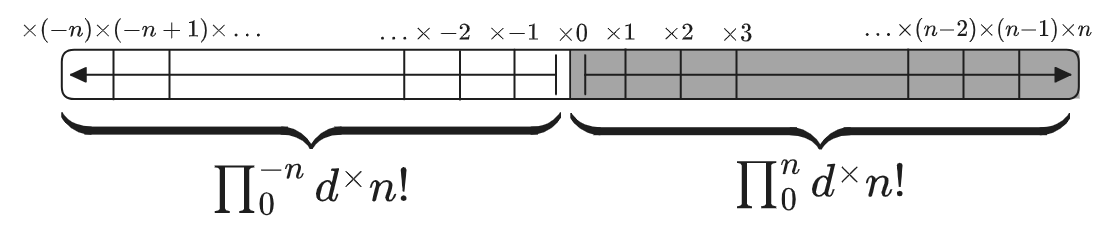
So we are interpolating a function that we only know one thing about—that going from \(n-1\) to \(n\) involves multiplying by \(n\)—and then we basically extrapolate from that fact, plus some assumptions, what it should do everywhere else. Since the integration range “starts” at \(0\) when going up, it “ends” at \(0\) going down, and we have to include the \(\times 0\) somewhere to go into the negatives, assuming the pattern holds. Since the integration range “ends” at \(\times n\) going up, it “ends” at \(\times (-n)\) going down, but since that’s the left side of an interval instead of the right side, we don’t include the \(\times (-n)\) in the product, which is why \((-n)!\) seems to make sense starting with the factor \(\times (-n+1)\) (or \(\times \frac{1}{(-n+1)}\), if you are doing the integral backwards, like the factorial seems to imply).

Note that it is probably also possible to identify \(n! \equiv \prod_{-\infty}^n d^{\times}(n!)\) and \((-n)! \equiv \prod_{-\infty}^{-n} d^{\times}(n!)\), if you assume that \(0! \equiv \prod_{-\infty}^0 d^{\times}(0!) = 1\) in some sense. But I would rather not try to not to assign a value to \(0!\) without having some geometric interpretation of what it’s supposed to mean in terms of permutation.

Also, just for the record, if ever we do have an interpretation in terms of permutations, it could certainly turn out to be the case that this generalization to \((-n)!\) is wrong. There’s really no way to say without having a sense of what it is actually supposed to be counting.

---

5. Negative Double Factorials

When you try to do that same expansion with double-factorials you quickly run into problems, which might make you think that the whole idea should be tossed out. One advantage of the product-integral interpretation of factorials is that it seems to fix the problems that arise, leaving intact the hunch that negative-integer factorials might be a valid concept.

Specifically, it seems like it should be true in some sense that \(1!! = 1 \times (-1) \times (-3) \times \ldots\) to infinity. Yet it is easy to find expressions using this that are clearly false based on this, for instance

\[\begin{aligned} 1 = \frac{1!!}{0!!} &\? \frac{1 \times (-1) \times (-3) \times (-5) \ldots}{0 \times (-2) \times (-4) \times (-6) \ldots} \\ &= \frac{1}{0} \times (\frac{1}{2}) \times (\frac{3}{4}) \times (\frac{5}{6}) \ldots \\ &= \frac{1}{0} \times \lim_{k \ra \infty} \frac{(2k-1)!!}{(2k)!!} \\ &\approx \frac{1}{0} \times \lim_{k \ra \infty} \frac{1}{\sqrt{\pi k}} \\ &\? \frac{1}{\sqrt{\pi}} \text{???} \end{aligned}\]

Writing each factorial as a product integral reveals that this computation was very flawed, however. It’s incorrect in the very first line

\[\begin{aligned} 1 = \frac{1!!}{0!!} &\? \frac{\prod^1_{-\infty} d^{\times}(x!!)}{\prod^0_{-\infty} d^{\times}(x!!)} = \prod_0^1 d^{\times}(x!!) = \sqrt{\frac{\pi}{2}} \text{ ???}\\ \end{aligned}\]

The problem is that the classical \(1!!\) is not \(\prod_0^1 d^{\times}(x!!) = 1!!/0!!\), but instead \(\prod_1^1 d^{\times}(x!!)\). Extending both factorials to infinity symmetrically requires including the missing \(\prod_0^1\) term as well.

\[\frac{1!!}{0!!} = \frac{\prod_1^1}{\prod_0^1} \times \frac{\prod_{-\infty}^0}{\prod_{-\infty}^0} = \frac{\prod_1^0 \prod_{-\infty}^1}{\prod_{-\infty}^0} = \frac{1}{\sqrt{\pi/2}} \frac{\prod_{-\infty}^1}{\prod_{-\infty}^0}\]

(omitting \(d^{\times}(x!!)\)s for brevity)

The deduction between the second and third lines is also wrong: it is not valid to write \(1!! = 1 \times (-1) \times (-3) \times \ldots = \lim_{k \ra \infty} (-1)^k (2k-1)!!\), because there is always a remainder term that that expression won’t include. We can tell because we know exactly what the partial products should be:

\[\begin{aligned} 1!!_{\text{new}} &= \sqrt{\frac{\pi}{2}} \\ (-1)!! &= (1!!_{\text{new}}) / (1) = \sqrt{\frac{\pi}{2}} \\ (-3)!! &= (-1)!!/(-1) = -\sqrt{\frac{\pi}{2}} \\ (-5)!! &= (-3)!!/(-3) = \frac{1}{3!!} \sqrt{\frac{\pi}{2}} \\ (-7)!! &= (-5)!!/(-5) = -\frac{1}{5!!} \sqrt{\frac{\pi}{2}} \\ 0!! &= 1 \\ (-2)!! &= (0)!!/(0) \? \infty \\ (-4)!! &= (-2)!!/(-2) \? -\frac{1}{2!!} \times \infty \\ (-6)!! &= (-4)!!/(-4) \? \frac{1}{4!!} \times \infty \\ \end{aligned}\]

(Where \(\infty = 1/0\) is being assumed to be somehow meaningful; we’re not even worried about that here.) So the actual values of the remainder at each point in the limit are

\[\begin{aligned} (-2k-1)!! &= \frac{(-1)^k}{(2k-1)!!} \sqrt{\frac{\pi}{2}} \\ (-2k-2)!! &= \frac{(-1)^k}{(2k)!!} \times \infty \end{aligned}\]

Which means the actual factorization of \(1!!/0!!\) is

\[\frac{1 \times (-1) \times (-3) \times (-5) \ldots}{0 \times (-2) \times (-4) \times (-6) \ldots} = \frac{1}{0} \times \lim_{k \ra \infty} \frac{(2k-1)!!}{(2k)!!} \times \frac{\frac{1}{(2k-1)!!} \sqrt{\frac{\pi}{2}}}{\frac{1}{(2k)!!} \times \infty} = \sqrt{\frac{\pi}{2}}\]

So it just doesn’t work: whatever partial product you construct, the remainder of the product just serves to cancel it all out again. Boring. Evidently, although you can extend factorials and double-factorials to negative infinity, it doesn’t really tell you anything you don’t already know: the value is fully determined by fixing it at \(n=0\).

I wish I knew what to make of the oscillating \(1/0 = \infty\) terms, though. My belief is that they are somehow perfectly meaningful, but I haven’t managed to find an interpretation that makes good sense of them yet. More on that later, maybe.

---

6. Multifactorials in general

It’s clearly possible to generalize all of this to higher-dimensional multifactorials, such as the triple factorial \(n!!! = n \times (n-3) \times \ldots\), the quadruple factorial \(n!!!!\), etc. Suppose we define \(F_1(x) = x!\) and \(F_2(x) = x!!\) and continue from there. We define that for all positive integers \(k\):

\[\begin{aligned} F_k(x) &= x \times (x-k) \\ F_k(0) &= 1 \\ \end{aligned}\]

This does not fully define \(F_k(x)\) completely on its own, of course, because knowing \(F_2(2)\), say, does not tell you anything about \(F_2(1)\) much less about \(F_2(3/2)\). But, extrapolating from the identity defining \(x!!_{\text{new}}\), we can also ask that \(F_k\) generally scales in \(k\) analogously:

\[\boxed{F_k(x) = k^{x/k} F_1(\frac{x}{k})}\]

That is, \(F_k(x)\) is just a rescaled version of \(F_1(x) = x!\), treating it as having exactly \(5/2\) “terms” in it. For example

\[\begin{aligned} F_2(5) = 5!!_{\text{new}} = 2^{5/2} (\frac{5}{2})! = 2^{5/2} F_1(\frac{5}{2}) \\ \end{aligned}\]

We can of course write any such function as an integral of its own derivative

\[F_k(n) = \frac{F_k(n)}{F_0(n)} \equiv \prod_0^n d^{\times} F_k(n)\]

Which means that the factorial over any range may be written as a ratio:

\[\frac{F_k(b)}{F_k(a)} = \prod_a^b d^{\times} F_k(n)\]

The difference between \(F_k(n)\) and \(n!!^{(k) \text{ times}}\), however, is the extrapolation of the difference between \((n!!)_{\text{old}}\) and \((n!!)_{\text{new}}\), which is that the “classical” double-factorial’s integration bound is offset

\[(kn+a)!!^{(k \text{ times})} \equiv \frac{F_k(kn+a)}{F_k(a-k)}\]

For instance

\[4!!!_{\text{old}} = (4) \times (1) \equiv \frac{4 \times 1 \times (-2)!!!}{(-2)!!!} = \prod_{-2}^4 d^{\times} F_3(x) = \frac{F_3(4)}{F_3(-2)}\]

Which means that \(F_k(n)\) and \((n)!!^{(k)}_{\text{old}}\) differ by a value of \(F_k(a)\) with \(a = n \mod k - k \in (-k, 0)\):

\[(kn+a)!!^{(k)}_{\text{old}} = \frac{F_k(kn+a)}{F_k(a - k)}\]

For example,

\[\begin{aligned} 6!!! &= \frac{6 \times 3 \times 0!!!}{0!!!} &= \frac{F_3(6)}{F_3(0)} &= 18 \\ 5!!! &= \frac{5 \times 2 \times (-1)!!!}{(-1)!!!} &= \frac{F_3(5)}{F_3(-1)} &= 10 \\ 4!!! &= \frac{4 \times 1 \times (-2)!!!}{(-2)!!!} &= \frac{F_3(4)}{F_3(-2)} &= 4 \\ \end{aligned}\]

Meaning that:

\[\begin{aligned} F_3(3) &= 3 \times F_3(0) = 3 \\ F_3(2) &= 2 \times F_3(-1) = 2 \times 3^{-1/3} F_1(-\frac{1}{3}) \\ &= 3^{-1/3} (-\frac{1}{3})! \\ &= 3^{-1/3} \Gamma(\frac{2}{3}) \\ F_3(1) &= 1 \times F_3(-2) = 1 \times 3^{-2/3} F_1(-\frac{2}{3}) \\ &= 3^{-1/3} (-\frac{2}{3})! \\ &= 3^{-1/3} \Gamma(\frac{1}{3}) \\ \end{aligned}\]

The value that corrects the double factorial of odd numbers, in particular, was

\[F_2(1) = F_2(-1) = 2^{1/2} F_1(\frac{1}{2}) = \sqrt{\frac{\pi}{2}}\]

Which is why

\[\begin{aligned} \frac{(2k+1)!!_{\text{new}}}{(2k+1)!!_{\text{old}}} &= \frac{\frac{F_2(2k+1)}{F_2(0)}}{\frac{F_2(2k+1)}{F_2(-1)}} \\ &= \frac{F_2(-1)}{F_2(0)} \\ &= F_2(-1) \\ &= \sqrt{\frac{\pi}{2}} \end{aligned}\]

Note that we don’t have to have \(F_k(0) = 1\) or any value at all really: the only thing we ever see are the relative values \(F_k(n)/F_k(0)\) anyway. All we have done here is follow the mindless construction of replacing a function \(f_k(x) = x!!!^{(k)}\) with \(F_k(x) = \prod_0^n d^{\times}(f+k(x)(x))\), which can be done for any function really, it has nothing to do with factorials per se. The argument for doing so is that the it compartmentalizes the odd behavior of the double-factorial: the discrepancy between \(x!!\) on even and odd numbers was completely and entirely due to the difference between \(F_2(-1)\) and \(F_2(0)\); other than that is it simply and mindlessly found by \(F_k(x) = k^{x/k} F_(x)\).

(This generalization is on Wikipedia also, but in a different notation. I prefer my way of thinking about it with integrals, though.)

Armed with this \(F_k(x)\), we can immediately write down such silly generalizations of the factorial as the “half”-factorial:

\[F_{1/2}(n) = n\times (n-\frac{1}{2}) \times (n-1) \times\ldots \times (1) \times (\frac{1}{2}) = 2^{-2n} F_1(2n)\]

For example

\[\begin{aligned} F_{1/2}(3) &= \frac{(3) \times \frac{5}{2} \times 2 \times \frac{3}{2} \times 1 \times \frac{1}{2} \times F_{1/2}(0)}{F_{1/2}(0)} \\ &= 2^{-6} \frac{6 \times 5 \times 4 \times 3 \times 2 \times 1 \times 0!}{0!} \\ &= 2^{-6} 6! \end{aligned}\]

Another thing we can try to do is to write down a “negative” factorial, which might look like a rising power instead of a falling one. But this gets awkward pretty quickly. Which of these should \(F_{-1}(n)\) equal?

\[\begin{aligned} F_{-1}(n) &\? n \times (n+1) \times (n+2) \times \ldots \\ &\stackrel{\text{or}}{=} (n+1) \times (n+2) \times (n+3) \times \ldots \\ &\stackrel{\text{or}}{=} (-1) \times (-2) \times (-3) \times \ldots (-n) \\ &\stackrel{\text{or}}{=} 0 \times (-1) \times (-2) \times \ldots (-n+1) \\ \end{aligned}\]

It depends whether you interpret \(F_k(n)\) as “start at \(n\) and go down \(k\) at a time” versus “start at \(0\) and go up \(k\) at a time”, and then additionally, whether things should be off by one if you’re going in the opposite direction. Maybe a reasonable thing to do is to attempt to get \(F_k(n) = k^{n/k} F_1(n/k)\) still hold.

But \(F_{-1}(n) = (-1)^{-n} F_1(-n)\) is kinda weird too, since \(F_1(-n) \? (-1)^{n-1}/(0 \times (n-1)!)\) is supposed to be that weird infinite negative factorial, which implies \(F_{-1}(n) = -1/(0 \times (n-1)!)\). The negative sign seems wrong, which makes me suspect this is not the right answer (although it seems to be there because we’re not considering the \(0\) as negative, which, it could be, because the whole thing is erroneously multiplying zero anyway). And even if you get over that, you’ll run into trouble with the other negatives: \(F_{-2}(n) = (-1)^{-n/2} F_1(-2n)\) is going to be multiplying each term by \(\pm i\), I suppose? What could that possible mean?

None of this matters that much. I really do suspect that there’s some valid meaning to \((-1)!\) and \(F_{-1}(1)\) and the others… but without an actual model of what these objects are supposed to be, it’s all just numerology. In every setting factorials are implicitly or explicitly connected to the cardinalities of permutations. For \((-1)!\) to be taken seriously, there must be an interpretation as the cardinality of a permutation of, like, a set with a negative number of elements, or something like that, and I’m not aware of such a thing.⁶

---

7. Euler’s Construction of \(\Gamma\)

One thing that I like about this \(F_k\) notation is that it organizes exactly what the “unusual” parts of multi-factorials are, after which the rest of their properties are trivial. In particular, other than the difference between \(1!! = F_{2}(1) / F_2(-1)\) and \(2!! = F_2(2)/F_2(0)\), multifactorials of all orders are exactly the same as rescaled single-factorials via \(F_k(n) = k^{n/k} F_1(n/k)\). So all of the behavior of \(F_k(n)\) for all \(k\) and \(n\) is fully defined by the values of \(F_1(x)\) on \(x \in (-1, 0)\), or equivalently, by \(\Gamma(z)\) for \(\text{Re}(z) \in (0,1)\).

Flipping that around: one might argue that the values of \(z!\) for \(z \in (-1, 0)\) would be defined by the asymptotic properties of the multifactorials. “What is \((-\frac{1}{2})! = \Gamma(1/2)\)”, you wonder? Well, it could be defined in order to make the multifactorials work out. Remember that

\[F_2(-1) \equiv \frac{(2k+1)!!_{\text{old}}}{(2k+1)!!_{\text{new}}} = \frac{(2k+1)!!_{\text{old}}}{F_2(2k+1)}\]

If we interpret things in this way, then the definition of \((-\frac{1}{2})!\) could be said to be

\[\begin{aligned} (-\frac{1}{2})! &= F_1(-\frac{1}{2}) \\ &\equiv 2^{1/2} F_2(-1) \\ &= 2^{1/2} \frac{(2k+1)!!_{\text{old}}}{F_2(2k+1)} \\ \end{aligned}\]

Of course, this is circular, since \(F_2(2k+1)\) is defined in terms of \(F_1(k+1/2)\) again

\[\begin{aligned} &\Ra 2^{1/2} \frac{(2k+1)!!_{\text{old}}}{F_2(2k+1)} \\ &= 2^{1/2} \frac{(2k+1)!!_{\text{old}}}{2^{k+1/2} F_1(k+1/2)} \\ &= \frac{(2k+1)!!_{\text{old}}}{2^k F_1(k+1/2)} \\ \end{aligned}\]

But it can also be taken as a limiting expression, which ends up matching a common construction of \(\Gamma\) due to Euler (see here). The argument goes: since for integers

\[(n + a)! \approx (n+1)^a n! \approx n^a n!\]

(Everyone writes this with \((n+1)^a\); I suppose that just makes it slightly more accurate.) Then we postulate that this ought to also hold for non-integer \(a\), in particular

\[(n+\frac{1}{2})! \approx (n+1)^{1/2} n! \approx (\sqrt{n}) n!\]

Then we define \((-1/2)!\) by approximating that denominator, and in the limit \(k \ra \infty\) it should become exact:

\[\begin{aligned} (-\frac{1}{2})! &\approx \frac{(2k+1)!!}{2^k (k+1/2)!} \\ &= \lim_{k \ra \infty} \frac{(2k+1)!!}{2^k k! \sqrt{k}} \end{aligned}\]

Which turns out to be \(\sqrt{\pi}\) (due to the Stirling’s Approximation; the \(\sqrt{\pi}\) ultimately shows up due to the Wallis Product, which I suppose is connected to \(n\)-spheres again).

I dunno. Maybe? I don’t find this construction much more philosophically satisfying than the others. It certainly doesn’t really “explain” how the \(\sqrt{\pi}\) gets there, it just phrases in terms of other things. But maybe it is a useful step to see it in this way: that the interpolated values of the factorial at fractions are explicitly equivalent to the ratio of a double factorial to a (rescaled) single-factorial. Maybe, then, the value comes fundamentally from something like “the ratio between a sphere of dimension \(2k+1\) and a tetrahedron of dimension \(k\)”. A “ratio of shapes”-type argument at least starts to suggest why the factors of \(\pi\) start to show up.

---

8. Interleaving Products

One other avenue of investigation.

As mentioned above, two double factorials can be interleaved to give one single-factorial.

\[(2k)!!_{\text{old}} (2k-1)!!_{\text{old}} = (2k)!\]

Obviously this is also possible for (standard) multifactorials of any order:

\[(4!!!)(3!!!)(2!!!) = (4 \times 1) (3) (2) = 4!\]

How do we understand this in terms of \(F_2(n)\)? In the new notation it becomes

\[\begin{aligned} (2k)!!_{\text{old}} (2k-1)!!_{\text{old}} &= \big[ \prod_0^{2k} d^{\times}(x!!)\big] \big[ \prod_{-1}^{2k-1} d^{\times}(x!!) \big] \\ &= 2^{2k} [\prod_0^{k} d^{\times}(x!)] [\prod_{-1/2}^{k-1/2} d^{\times}(x!)] \end{aligned}\]

To figure out how to make equal to \((2k)!\), consider an example:

\[\begin{aligned} (6!!_{\text{old}})(5!!_{\text{old}}) &= (6 \times 4 \times 2) \times (5 \times 3 \times 1) \\ &= 2^3 (3 \times 2 \times 1) \times 2^{3} (\frac{5}{2} \times \frac{3}{2} \times \frac{1}{2}) \\ &= 2^{6} (\frac{6}{2} \times \frac{5}{2} \times \frac{4}{2} \times \frac{3}{2} \times \frac{2}{2} \times \frac{1}{2}) \end{aligned}\]

Which is a “half” factorial. So double factorials interleave to give single factorials, or single factorials interleave to give half factorials (times an awkward extra factor). Fine.

\[\begin{aligned} (6!!_{\text{old}})(5!!_{\text{old}}) &= (6 \times 4 \times 2) \times (5 \times 3 \times 1) \\ &= 6 \times 5 \times 4 \times 3 \times 2 \times 1 \\ &= 6! = F_1(6) \\ &\equiv \frac{F_1(6)}{F_1(0)}\\ (3!)(\frac{5}{2}!) &= (\frac{6}{2} \times \frac{4}{2} \times \frac{2}{2}) \times (\frac{5}{2}\times \frac{3}{2} \times \frac{1}{2} \times (-\frac{1}{2})!) \\[10pt] &= \frac{6}{2} \times \frac{5}{2} \times \frac{4}{2} \times \frac{3}{2} \times \frac{2}{2} \times \frac{1}{2} \times (-\frac{1}{2})!\\ &= F_{1/2}(3) \times F_1(-\frac{1}{2})\\ &\equiv \frac{F_{1/2}(3)}{F_{1/2}(0)} F_1(-\frac{1}{2}) \end{aligned}\]

Therefore the interleaving property for double factorials can be written:

\[\frac{F_2(n)}{F_2(0)} \frac{F_2(n-1)}{F_2(-1)} = \frac{F_1(n)}{F_1(0)}\]

And the half-factorial version:

\[\frac{F_1(n)}{F_1(0)} \frac{F_1(n-\frac{1}{2})}{F_1(-\frac{1}{2})} = \frac{F_{1/2}(n)}{F_{1/2}(0)}\]

Plugging in \(F_k(n) = k^{n/k} F_1(n/k)\) recovers the Legendre duplication formula again:

\[\begin{aligned} n! (n-\frac{1}{2})! &= F_1(n) F_1(n-\frac{1}{2}) \\ &= F_{1/2} (n) F_1(-\frac{1}{2})\\ &= \frac{1}{2^{2n}} F_1(2n) F_1(-\frac{1}{2}) \\ &= \frac{(2n)!}{2^{2n}} \sqrt{\pi} \end{aligned}\]

A natural thing to do is to generalize this to \(k\)-factorials. For example, when \(k=3\), we can obviously interleave three factors instead of two:

\[\begin{aligned} (3n)! &= (3n)!!! \times (3n-1)!!! \times (3n-2)!!! \end{aligned}\]

Which we write as

\[\begin{aligned} (3n)! &= \frac{F_3(3n)}{F_3(0)} \times \frac{F_3(3n-1)}{F_3(-1)} \times \frac{F_3(3n-2)}{F_3(-2)}\\ \end{aligned}\]

Rearranging :

\[\begin{aligned} (3n)! &= 3^{3n} \frac{F_1(n) F_1(n-\frac{1}{3}) F_1(n- \frac{2}{3})}{ F_1(0) F_1(-\frac{1}{3}) F_1(-\frac{2}{3})} \\ \end{aligned}\]

Which an equation for the interleaved \(1\)-factorials offset by \(\frac{1}{k}\), in terms of a product of values of \(x!\) in \((-1, 0)\)

\[F_1(n) F_1(n-\frac{1}{3}) F_1(n- \frac{2}{3}) = \frac{(3n)!}{3^{3n}} F_1(-\frac{1}{3}) F_1(-\frac{2}{3})\]

So once again, all of the structure of \(x!\) and \(F_k(x)\) seems to come from the values in that interval. The general case takes products of \(k\) factorials to a single \((kn)\) factorial times some coefficients:

\[\prod_{j=0}^{k-1} F_1(n - \frac{j}{k}) = \frac{(kn)!}{k^{kn}} \prod_{j=0}^{k-1} F_1(-\frac{j}{k})\]

It is possible to simplify this further by finding the value of the product on the RHS giving the “Gauss Multiplication Formula”, but the technique is much less simple than the algebraic manipulations we’ve been doing so far. It’s not very satisfying, but I’ll include it for completeness. This version comes from Artin’s tiny book on the Gamma function. I’ve translated the notation from \(\Gamma\) back to factorials (which makes it a bit simpler to read, also…); some other proofs can be found here.

However you define \(x!\), it must be that

\[(x+m)! = x! (x+1)(x+2) \cdots (x+m)\]

And also that

\[(x+m)! = m! (m+1) (m+2) \cdots (m+x)\]

Since both hold as \(m \ra \infty\) and (we postulate) should hold for non-integer \(x\), we rearrange things to get an approximation for a non-integer factorial \(x!\) in terms of an integer factorial \(m!\) when \(m \gg x\). We use the approximation \((m+x)! \approx m^x m!\):

\[\begin{aligned} x! &\approx \frac{(x+m)!}{(x+1)(x+2) \cdots (x+m)} \\[2ex] &\approx \frac{m^x m!}{(x+1)(x+2) \cdots (x+m)} \\[2ex] &= \lim_{m \ra \infty} \frac{m^x m!}{(x+1)(x+2) \cdots (x+m)} \end{aligned}\]

In this form we can compute that product, because when we multiply this together for every \(F_1(-\frac{j}{k})\), the denominators interleave to form a single giant factorial, and the numerators can be grouped together via \(\prod m^{-j/k} = m^{-[0+1+2+\ldots+k-1]/k} = m^{-k(k-1)/2k} = m^{-(k-1)/2}\). The algebra is hard to watch:

\[\begin{aligned} \prod_{j=0}^{k-1} (-\frac{j}{k})! &= \lim_{m \ra \infty} \prod_{j=0}^{k-1} \frac{m^{-j/k} m!}{(-\frac{j}{k}+1)(-\frac{j}{k}+2) \cdots (-\frac{j}{k}+m)} \\ &= \lim_{m \ra \infty} \prod_{j=0}^{k-1} \frac{k^m m^{-j/k} m!}{(-j+k)(-j+2k) \cdots (-j+km)} \\ &= \lim_{m \ra \infty} \frac{k^{km} m^{-(k-1)/2} (m!)^k}{(km)!} \end{aligned}\]

But eventually plugging in Stirling’s approximation miraculously cancels out all the \(m\)s, as it ought to:

\[\begin{aligned} \prod_{j=0}^{k-1} (-\frac{j}{k})! &= \lim_{m \ra \infty} \frac{\cancel{k^{km}} m^{-(k-1)/2} (\sqrt{2 \pi m})^k \cancel{(m/e)^{km}}}{\sqrt{2 \pi k m} \cancel{(km/e)^{km}}} \\ &= \lim_{m \ra \infty} \frac{m^{1/2 - k/2 + k/2 - 1/2} (2\pi)^{k/2 - 1/2}}{k^{1/2}} \\ &= (2 \pi)^{(k-1)/2} k^{-1/2} \end{aligned}\]

Which finally gives the general rule for interleaved factorials, the Gauss Multiplication Formula (which is normally written slightly differently, of course)

\[\begin{aligned} \prod_{j=0}^{k-1} (n-\frac{j}{k})! &= (2 \pi)^{\frac{k-1}{2}} k^{-kn -\frac{1}{2}} (kn)! \\ &= \frac{(2 \pi)^{\frac{k-1}{2}}}{\sqrt{k}} \frac{(kn)!}{k^{kn}} \end{aligned}\]

For the \(k=3\) example, this is

\[n!!! \times (n - \frac{1}{3})!!! \times (n-\frac{2}{3})!!! = \frac{2 \pi}{\sqrt{3}} \frac{(3n)!}{3^{3n}}\]

The \(2 \pi / \sqrt{3}\) factor is the only non-trivial part; the other term just comes from \(F_k(n) = k^{n/k} F_1(n/k)\).

---

9. Ending

This is all very tedious. The reason for going through it at all is that there is some kind of curious structure here that I’m trying to tease out. It is weird, of course, that \((-1/2)! = \sqrt{\pi}\). But it also weird that products of more fractions, such as \((-1/3)!(-2/3)!\), end up proportional to \(2\pi^{(k-1)/2}\). Whatever mysterious interpretation is out there for fractional factorials that connects them (presumably) to fractional ‘sets’ and fractional ‘permutations’… it needs to explain this behavior. Why do products of fractions cancel out to give factors of \(\pi\)? In what way are we “factoring” spheres when we evaluate \(x!\) on a fraction? These are questions that as far as I know are unanswered, and are possibly silly, but they don’t seem that silly; there has got to be some kind of geometric structure underlying this that is more satisfying than “it is the log-convex interpolation of \(x!\)” or “it is the analytic continuation of \(x!\)” or “it’s what you get by manipulating a bunch of infinite products” or whatever.

In any case it is clear that multifactorials are closely related to regular factorials/Gamma functions, times some coefficients, and all the interesting behavior shows up in the definitions of \(x!\) on \((-1, 0)\), or equivalently \(\Gamma\) on \((0,1)\). (See also the multifactorial stuff on here, which is presumably equivalent to how I’ve done things here.)

By the way: a lot of these identities are not really factorial-specific; they’re all true of any family of sequences, such as summations, products, or whatever else. The identity for interleaving double-factorials expresses the same thing, up to some logarithms, as

\[\sum_{i=0, \text{ even}}^{2k} S_i + \sum_{i = -1, \text{ odd}}^{2k-1} S_i = \sum_{i = -1}^{n} S_i\]

And the general operation of interpolating sequences to non-integers is not really factorial-specific either. starting with \(f(n)\) defined on non-integers, to compute \(f(x)\) for non-integer \(x\) you:

1. Find the asymptotic behavior \(\lim_{n \ra \infty} f(n)\)
2. Assume that the asymptotics hold for \(f(n+x)\)
3. Compute \(f(x) = f(n)^{-1} \circ f(n+x)\) and call this the value of \(f(x)\), where the inverse could be addition, multiplication, or whatever you want.

As far as I can tell this is what \(\Gamma\) is doing, and when you put it like this it’s kind of a hard sell to say that it means something at all, given that the result you get is very specific on how you parameterize \(f\) (changes of variables will give different answers, I mean). Except, of course, for the fact that the \(n\)-spheres have \(\Gamma\)s in their volumes! That’s really what ties it all together—we have “experimental evidence” (of a sort) that this process gives something meaningful in the case of \(n!\), so we’re forced to take it seriously. Curious.

Incidentally this way of interpolation has been studied; I’m aware of a somewhat-obscure theory of interpolating infinite sums and there are plenty of other references to people looking into it. I hope to study it in more detail later but this is long enough and my brain hurts.

By the way, the most important thing that I have not looked into yet is the “reflection” identity for \(\Gamma\),

\[\Gamma(z) \Gamma(1-z) = \frac{\pi}{\sin \pi z}\]

And I do think that this might be the key to unlocking everything. There is a nice way to rewrite it (…once you drop the \(\Gamma\) notation. I keep feeling like thy’re just getting in the way of everything…) as

\[(z)! (-z)! = \frac{\pi z}{\sin \pi z} = i \frac{(\pi z) - (-\pi z)}{e^{i \pi z} - e^{-i \pi z}}\]

Which seems to imply some structure: it’s the ratio of (a difference of translations by \(\pi z\)) to (a difference of rotations by \(\pi z\)). Which feels like an important clue. Perhaps it is also related to the interpretation of \(\Gamma\) as an integral transform against the Haar measure \(d(\ln x)\). If a factorial is (something like) a change-of-basis coefficient between \(\bb{R}^+\) and \(\bb{R}^{\times}\), but then we interpolate \(\bb{R}^{\times}\) into rotations, then… I don’t know… maybe that explains how it ends up dealing with \(\sqrt{\pi}\) or factorizations of it? Gosh, I have no idea, I’m completely lost.

One thing is for sure. No number of complex-analytic factoids about the continuation of \(\Gamma\) are going to settle all this. Some kind of philosophical model of what it means to interpolate between permutations is going to have to show up, eventually, somewhere, and that probably means contending with something that acts like a fractional set.