Exterior Algebra #6: Oriented Projective Geometry

February 23, 2019

In the previous post in this series, I looked at how some operations related to exterior algebra (wedge / ‘join’, ‘meet’, interior product, Hodge Star, geometric product) roughly correspond to set operations (union, intersection, subtraction, complement, symmetric difference), but the analogy wasn’t very good. Exterior algebra isn’t exactly linearized set algebra. So what is it?

Well, I found another subject that’s a much closer fit: oriented projective geometry (henceforth ‘OPG’).

OPG is the mathematics of oriented figures in space – ‘positive’ and ‘negative’ points, lines with directions, planes with orientations, etc, along with operations like “finding the line between two points” and “determining which side of a line a point is on”. It turns out that every operation in OPG is exactly the same as one in exterior algebra, except that in OPG everything is defined up to multiplication by a positive scalar. OPG is exterior algebra if you forget about all the magnitudes scalars.

I read through the book “Oriented Projective Geometry” by Jorge Stolfi (1991), which is very readable and interesting though it could really use more concrete examples. Stolfi was at least aware of the relationship with exterior algebra also, and he cited the same Barnabei/Brini/Rota paper I’ve been looking at in previous posts. Some of his terminology and notation is better than that in EA and some is worse. In this article I to summarize the main ideas of OPG and compare it the exterior algebra that I’ve been studying.

1. Exposition

Oriented projective geometry is a way of doing analytical geometry in \(n\)-dimensional space that has mathematical representations of points, lines, planes, etc.

We start with \(\bb{R}^n\) and construct an “oriented projective space”¹ \(\bb{O}^n\). Its objects are oriented points, lines, and planes. Oriented points can point into or out ‘of the page’. Oriented lines have a direction; oriented planes have an orientation, defined by choosing a normal vector that says which way is “up”. Conceptually, there are two copies of \(\bb{R}^n\) overlaid, one of positive points and one of negative points. For any point \(p\), we can denote its negatively-oriented counterpart (called its antipode) as \(\neg p\).

For points this means we have both \(a\) and \(\neg a\). I tend to think of one as “going into the page” and the other as “coming out of the page”, although this intuition is admittedly thin — it is mostly for symmetry with all the other oriented objects. For lines, \(l\) and \(\neg l\) refer to the same line but traversed in the opposite directions. This is useful, for instance, for saying if a point is on the left or right side of a line: for that to make sense, we have to be able to say which direction the line is pointing. Later on if we were to construct, say, polygons, we’d say that each side is an oriented line segment from a negative point to a positive point. That sort of thng.

In each case there are two copies of every object (point, line, etc), one of each orientation. We might imagine each \(\bb{O}^n\) as constructed from two copies of \(\bb{R}^n\), glued together at their infinities.

Examples:

\(\bb{O}^0\) is just two points, with opposite orientations.

\(\bb{O}^1\) is two copies of the real line, with the positive infinities of each linked to the negative infinities of the other, resulting in a topological circle:

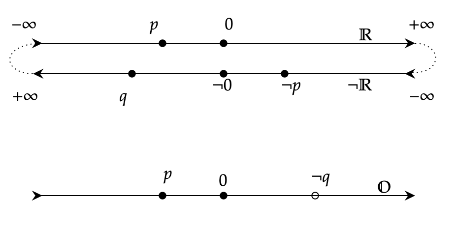
\(\bb{O}^2\) is two copies of the real plane, which we may picture as being spread over two hemispheres of a sphere, with antipodal points being oppositely oriented (hence the name ‘antipode’), and the equator that joins them as the line at infinity.

\(\bb{O}^3\) is two copies of Euclidean space, joined together at infinity so that \((x,y,z) \times \infty\) is the same point as \(\neg (-x, -y, -z) \times \infty\). You’ll just have to find your own way to visualize it. \(\b{O}^3\) contains a pair of oriented volumes which basically correspond to right-handed and left-handed coordinate systems.

In each case the two spaces are connected by a “horizon” or “hyperplane at infinity” which causes directions to “wrap around”: \(+ \infty = \neg (- \infty)\). In \(\bb{O}^1\) the two real lines are glued together by two points, a copy of \(\bb{O}^0\). In \(\bb{O}^2\), the line at infinity is a circle, a copy of \(\bb{O}^1\), which glues the ‘borders’ of two planes together, etc. Evidently each \(\bb{O}^n\) is topologically equivalent to an \(n\)-sphere, and its line at infinity is a copy of \(\bb{O}^{n-1}\), an \((n-1)\)-sphere. For comparison, regular projective geometry, without the word “oriented”, refers to the same structure but with each point identified with its antipode, which causes it to have very strange topological properties that I have personally no interest in dealing with.

Why do any of this? Basically because it turns out to be useful when dealing with properties of oriented geometric objects. If you are considering the geometric relationships of oriented shapes, like “lines with directions” or “clockwise circles”, you are already working with these sorts of concepts. Oriented objects turn out to be a good representation for answering questions like “what side of a line is a point on?” or “is a point contained in figure?” or “what is the intersection of two planes?”, and is ubiquitous (in one form or another) in computer graphics and anything else dealing with representing spatial geometry.

Homogenous Coordinates

The simplest representation of the points of \(\bb{O}^n\) is as directions in \(\bb{R}^{n+1}\), which are called homogenous coordinates.

The standard way of picturing this is easy to visualize in \(\bb{R}^3\). Picture a distinguished plane, called \(P\), which is positioned at \(z=1\). First we’ll describe homogenous coordinates in unoriented projective geometry:

Lines in \(\bb{R}^3\) wll correspond to points according to where they intersect \(P\). A vector \((a,b,c)\) corresponds to the point \((a/c, b/c, 1)\), because by dividing out the \(z\) coordinate we’re left with its position on the \(P\) plane.
Lines in \(\bb{R}^3\) can also be treated as the normal of a plane. The intersection of a plane with \(P\) gives a line. If we create that normal direction by taking the cross product of two other directions \(\b{a} \times \b{b}\), the resulting plane is the plane that goes between those two points.
Points with \(z=0\), like \((a,b,0)\), never intersect the \(P\) plane. We regard these as “points at infinity” on the plane — it’s the infinitely-distant point \((a,b)\). Alternatively, you can imagine that the \(z=0\) is actually just a very small number, like \(z = \e\), so the point is put as far away as you want.
Any nonzero multiple of a point, like \((\lambda a, \lambda b, \lambda c)\), corresponds to the same point, since \((\frac{\lambda a}{\lambda c}, \frac{\lambda b}{\lambda c}, 1) = (a/c, b/c, 1)\). So, a point on \(P\) is really an equivalence class of vectors in \(\bb{R}^3\).

This construction is normally used to define points in unoriented projective geometry. In oriented projetive geometry, the difference is that points are only the same point if they differ by a positive scalar. For instance \((2a, 2b, 2c) = (a,b,c)\), but \((-a, -b, -c) \neq (a,b,c)\). This means that points on \(P\) correspond to rays in \(\bb{R}^3\), rather than lines.

So, a point in \(\bb{O}^n\) is defined as equivalence class of vectors in \(\bb{R}^{n+1}\), where two vectors are equivalent if they differ by positive scalar factor. The positive scalar factors are what make our objects oriented. If \((a,b,c)\) corresponds to the point \((a/c, b/c)\) in \(\bb{O}^2\), then \((-a, -b, -c)\) corresponds to the point \(\neg (a/c, b/c)\) — the same point, just oppositely oriented.

These refer to the same point in \(\bb{O}^2\), assuming all three \((a,b,c)\) are positive:

\[(a,b,c) = (2a,2b,2c) = (a/c, b/c, 1) = (1, b/a, c/a) = (a/b, 1, c/b)\]

As long as \(c \neq 0\), this is still the same point:

\[(a,b,c) = (a / | c |, b / |c|, \sgn(c), )\]

These are all different points, though:

\[(a,b,c) \neq (a, b, -c) \neq (-a, -b, -c) \neq (a/c, b/c, 0)\]

Clearly the relevant information to define a point in \(\bb{O}^2\) is two real numbers \((x,y)\) and a ‘sign flag’, which can be \(\{+1, 0, -1\}\). It’s often easiest to just not divide through, when doing calculations, to avoid having to be careful about signs and absolute values.

\[(x,y, \sgn) \in \bb{O}^2\]

\(\sgn = +1\) refers to ‘positive points’, \(\sgn = -1\) to ‘negative points’, and \(\sgn = 0\) to points at infinity in the direction of \((x,y)\). This means that \((x,y, 0) \sim ( x/y, 1, 0)\) also, which incidentally shows that the hyperplane at infinity in \(\bb{O}^n\) is itself a copy of \(\bb{O}^{n-1}\).

To visualize this embedding for, say, \(\bb{O}^1\): consider the real plane \(\bb{R}^2\) with vertical lines drawn at \(x=1\) and \(x=-1\), which will be the “front” and “back” parts of \(\bb{O}^1\). Points in \(\bb{O}^1\) correspond to “directions” in \(\bb{R}^2\), which are determined by taking vectors \((x,y)\) and seeing where they intersect one of the two vertical lines. If \(y > 0\), the intersection point is \((1, x/y)\), on the front line; if \(y < 0\), the point is \((-1, x/y)\) on the “back line”. Like this:

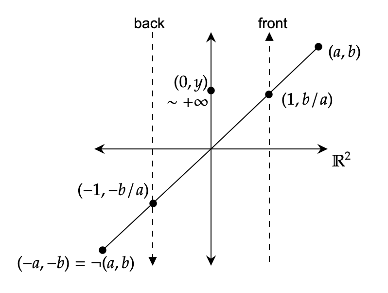
The point \((0, x)\) maps to \(+\infty\), which is the same as \(\neg (-\infty)\), if \(x > 0\) and \(-\infty\) if \(x < 0\). The point \((0,0) \in \bb{R}^2\) doesn’t correspond to anything in \(\bb{O}^1\), and is considered undefined or null.

With a bit of work you learn to think in this model. In linear algebra we tend to regard every direction from the origin as a unique ‘direction’. In OPG we regard every point as a unique direction (say, from your eyes); their spans are lines/planes/higher-dimensional analogues (called ‘affine subspaces’) which contain them, and linear independence is when they aren’t contained in the same line/plane/affine subspace.

Basically: when talking about the geometry of shapes, the origin really isn’t special, and thus we do geometry in a way that doesn’t privilege it.

Flats and Simplexes

In OPG an oriented hypersurface is called a ‘flat’: an oriented point, line, plane, etc. For each flat \(a\) is there is an opposite flat, written \(\neg a\), consisting of the same object with the opposite orientation. A flat’s rank is how many points are required to define it: a point has rank \(1\), a line rank \(2\), etc (it’s the dimension of the figure plus one, or the dimension of the figure in the \(\bb{R}^{n+1}\) model). We’ll refer to flats of rank \(k\) as \(k\)-flats. There are also two “empty” flats of rank \(0\), called \(\Lambda\) and \(\neg \Lambda\), which are like oriented empty sets.

A simplex is a list of points, written \((abc\ldots)\). A proper simplex is one whose points are linearly independent, which means that the simplex does not contain any duplicates, copies of the same point with opposite orientations, sets of three collinear points, etc. This is necessary to determine a flat uniquely: two points to determine a line, three for a plane, etc. Linear independence rules out calling \((a,a,b)\) a plane or \((p, \neg p)\) a line. We’ll almost always just say ‘simplex’ when we mean ‘proper simplex’ because we don’t care about improper simplexes.

A proper \(k\)-simplex has \(k+1\) points in it, because it determines a \(k\)-flat – so a \(0\)-simplex is a point, a \(1\)-simplex is a line, etc. This turns out to be a lot less confusing than if a \(k\)-simplex were to have \(k\)-points in it.

Basically, flats are oriented \(k\)-surfaces and proper simplexes are oriented \(k\)-segments (line segments, triangles, tetrahedrons, etc). Flats are usually the objects of study, but may be referred to by any simplex which defines them, and computations take place with a choice of simplex and should give the same result for any valid choice of simplex for each flat.

The \(\neg\) symbol reverses orientations of simplexes, and acts sort of like a minus sign. In the vector representation of points, it literally is one: \(\neg(x,y, 1) = (-x,-y, -1)\). Negating a simplex negates the orientation flat it refers to. The same representation can be reached by swapping any two of its points, or negating all of them:

\[\begin{aligned} (p,q) &= (\neg p, \neg q) \\ &= \neg (q, p) \\ &= \neg (\neg q, \neg p) \end{aligned}\]

Operations on Flats

Flats support the operation of join \(\v\). Join just appends the simplex representations as lists, so long as none of the points lay in the same hyperplane as the others (ie, \(k+1\) points describes either a \(k\)-dimensional figure or an “empty” simplex.). For example:

\[(p,q) \v (r,s) = \begin{cases} (p,q,r,s) & \if p,q,r,s \text{ linearly independent} \\ 0 & \text{ otherwise} \end{cases}\]

The join operation is associative and “rank commutative”:

\[\begin{aligned} p \v (q \v r) &= (p \v q) \v r = p \v q \v r \\ p \v q &= \neg^{\text{rank}(p)\text{rank}(q)} q \v p \end{aligned}\]

Which side of \(\bb{O}^n\) is the ‘positive’ side may be specified by supplying a global orientation flat \(\Omega\), also called a ‘universe’, which is any oriented \(n\)-flat (there are only two choices anyway).

Flats also support the operation of meet \(\^\) relative to the global orientation, which is an oriented version of intersection. It’s given by:

\[\begin{aligned} \alpha \^ \beta &= \begin{cases} q & \exists\, p, q, r : \\ & p \v q \v r = \Omega \\ & p \v q = \alpha, q \v r = \beta \\ 0 & \text{ otherwise} \end{cases} \end{aligned}\]

Meet is associative and “corank commutative”, where the “corank” of a simplex in \(\bb{O}^n\) is \(\text{corank}(p) = \text{rank}(\Omega) - \text{rank}(p) = (n+1) - \text{rank}(p)\).
:

\[\begin{aligned} p \^ (q \^ r) &= (p \^ q) \^ r = p \^ q \^ r \\ p \^ q &= \neg^{\text{corank}(p) \text{corank}(q)} q \^ p \\ \end{aligned}\]

The complement of a flat \(x\), written \(x^{\perp}\), is a flat \(y\) such that \(x \v y = \Omega\), and of course \(\text{rank}(x^{\perp}) = \text{corank}(x)\). If a flat \(x\) is contained in a flat \(f\), we can also define the complement with respect to \(f\) as a flat \(y\) such that:

\[x^{\perp f} = \begin{cases} y & \exists \, y : x \v y = f \\ 0 & \text{ otherwise} \end{cases}\]

Summarizing

This is all exactly the same as exterior algebra. Well, up to a positive scalar factor, and the fact that the symbols \(\^\) and \(\vee\) are swapped.

Simplexes are the same objects as multivectors. Each point in space corresponds to a vector, and higher-grade multivectors correspond to the geometric objects spanned by their points. \(\neg\) is multiplication by \(-1\). Joins (written \(\v\) in OPG) are wedge products (written \(\^\) in EA). Meets \(\^\) are meets \(\v\). \(\Omega\) is \(\omega\). Complements are Hodge Stars and interior products. \(\text{corank}(p)\) is \(\| {\star p} \|\).

So that’s fun.

(By the way, so we don’t get confused, in this article \(\v\) will refer to the join/wedge product (what I normally write \(\^\)) and \(\^\) will refer to the meet. That’s probably what exterior algebra should use, but it’s too late to change.)

Note that it’s the vector representation in \(\bb{R}^{n+1}\) that is isomorphic to EA. I like to use the unit vector \(\b{w}\) as the basis for the additional coordinate. For instance the simplex created by \((2 \b{x}, \b{y})\) is equivalent to the multivector

\[(\b{w} + 2 \b{x}) \vee (\b{w} + \b{y}) = (1,2,0) \v (1,0,1) = (-2,2,-1) \sim (-1, 1, -\frac{1}{2})\]

and not \((2,0) \v (0,1) = 2 \b{x \v y}\).

In OPG, vectors describe points and the join of two points (vectors) is a line (bivector). In EA, vectors describe lines, and the join of two points is a plane (bivector). So the EA on a vector space \(\bb{R}^n\) is equivalent to the OPG \(\bb{O}^{n-1}\). But the arithmetic is all the same, and we could represent \(k\)-simplexes, rather than by a list of \(k\) points \((p,q,\ldots)\), by a single \(k\)-vector in \(\^^k \bb{R}^n\) – although this would almost always require storing more data; multivectors are not at all an efficient way to store information. Usually storing a list of vectors is a better idea.

Some connections to other stuff: what we’ve called a flat is also called (though the definitions usually don’t include orientation) an “affine subspace” or “linear variety”, and \(\bb{O}^n\) is an affine space, which is the name for a Euclidean space where we have no special concept of an origin. If we forgot about the requirement that our scalar factors be positive (and did away with the \(\neg\) sign) we would be working in standard projective geometry, but the oriented version of projective geometry, while less common is necessary if we want properties like the anticommutativity of join to line up with those in exterior algebra.

Projective geometry deals with many of the same objects in a slightly different way; IMO it is often doing the same thing but with a lot of confusion about what’s going on. There is a thing called the Grassmannnian \(\text{Gr}_k(V)\) of a vector space \(V\), which is the set of all \(k\)-linear subspaces of \(V\) (regarded as a manifold, I guess). The elements of the Grassmannian are mapped to multivectors by the Plücker Embedding, with coordinates called Plücker Coordinates (or “Grassmann coordinates”).

Good Ideas from OPG

There are a few things in Stolfi’s book that I think are obviously good and worth importing into my understanding of EA (and some things obviously missing from OPG that EA knows about, but I’m not as concerned with that direction).

1. It is useful to define meets with respect to any set, not just the whole vector space. The “meet of \(a\) and \(b\) in \(u\)” is a multivector \(y\) such that there exist multivectors \(x,z\) with:

\[\begin{aligned} x \v y \v z &= u \\ x \v y &= a \\ y \v z &= b \end{aligned}\]

Then \(y = a \^_u b\). (This is probably a better way to intuit what the meet does, anyway; I should have maybe written it this way last time…) \(u\) has to be spanned by \(a\) and \(b\), and \(y\) is their ‘overlap’. The regular meet operation is just this generalized meet with respect to the universe/pseudoscalar: \(a \^ b \equiv a \^_{\Omega} b\).

The commutativity law now uses coranks “relative to \(u\)”:

\[a \^ b = \neg^{\text{corank}_u(a) \text{corank}_u(b)} b \^ a\]

By the way, \(x^{\perp}\) is definitely a better notation than \(\star x\). Though it is helpful to have it as a prefix operator, so maybe we should write it as \(\perp x\). And capital omega \(\Omega\), which really looks like “omega” and evokes feelings of “finality” and “totality”, is definitely better than lower-case omega \(\omega\), which just looks like a weak “w”. And the name “universe” is definitely better than “pseudoscalar”.

2. We can also define joins with respect to any flat/multivector. This one is a bit weirder. Basically, if you have two flats (multivectors) \(v \v x\) and \(v \v y\), you can define their “join relative to \(v\)” (“relative join”), as:

\[(v \v x) \v_v (v \v y) = v \v x \v y\]

This is the dual operation to the “meet in a flat”. We write it as \(\alpha \v_v \beta\), and we can compute it (with \(v^{-1} = \frac{v}{\| v^2 \|}\)):

\[\alpha \v_v \beta = (v^{-1} \cdot \alpha) \v \beta = \alpha \v (v^{-1} \cdot\beta )\]

3: Remember how \(\v{\^} V\) is the “double” algebra, consisting of two exterior algebras over the same basis multivectors space? In fact, this can be made much more general.

Let us write an exterior algebra as a tuple of a vector space and a join operation. The standard exterior algebra is \((\bb{R}^n, \v)\). The ‘meet’ algebra is \((\^^{n-1} \bb{R}^n, \^)\). The double algebra refers to both at once, which we may write as \((\bb{R}^n, \v, \^)\).

Let \(S_\alpha\) be the space of multivectors contained in \(\alpha\), for example in \(\bb{R}^3\), \(S_{\b{x \v y}}\) is the \(\b{x \v y}\) plane consisting of all multivectors with no \(\b{z}\) component. Then \((S_\alpha, \v)\) is an exterior algebra for any \(\alpha \in \^ \bb{R}^n\), isomorphic to \(\^\bb{R}^{\| \alpha \|}\), and \((S_\alpha, \v, \^_\alpha)\) is a double algebra in the same way.

Moreover, given any two multivectors \(\alpha, \beta\) with \(\beta \in S_{\alpha}\), we can define an exterior algebra and double algebra “between them”, using the relative-join, so \((S_{\alpha}, \v_{\beta}, \^_{\alpha})\) is a double algebra also. This strikes me as very cool. But also confusing.

I am not even sure what that would look like. As an example consider the 2-dimensional space spanned by \((\b{x \v y}, \b{x \v z})\) inside of the 4-dimensional space spanned by \(\Omega = \b{w \v x \v y \v z}\), where we take joins relative to \(\b{x}\): \((\b{x \v y}) \v_{\b{x}} (\b{x \v z}) = \b{x \v y \v z}\) and meets relative to \(\Omega\): \((\b{x \v y \v z}) \^_{\Omega} (\b{x \v z \v w}) = (\b{x \v z})\).

Something I often think about: perhaps one of the transformations that a geometric calculus should be invariant under is the operation of “forgetting about dimensions”. In this case, we see that the exterior algebra on \(\bb{R}^4\) remains an exterior algebra if we just ‘forget about \(\b{x}\)’ entirely, either by literally projecting every object onto the \(\b{y \^ z \^ w}\) plane, or – as we’ve done here – by defining operations that just pretend like it isn’t there.

4: OPG points out that it is useful (especially in computer implementations) to distinguish between the \(0\)s in different vector spaces. In EA terms, this means that the \(0 \in \bb{R} \simeq \^^0 V\) is not the same as \(0 \in \^^{2} V\); we can distinguish them by writing \(0^k\) for the element of \(\^^k V\). I think this is a good idea. \(0^{\v k}\) would be good also.

5: OPG has a useful operation I hadn’t thought to write down: a boolean function for determining “relative sign” of two complementary flats / multivectors. For two multivectors \(\alpha, \beta \in \v V\) with \(\| \alpha \| + \| \beta \| = n = \dim V\), we write:

\[\alpha \diamond \beta = \sgn(\alpha \v \beta)\]

(Recall that \(\sgn\) gives 0 if its argument is \(0\). We of course also take it to be \(0\) if its argument is any \(0^k\), in the notation of the previous section.)

This is useful for answering questions about the relative orientations of objects. If we have a point \((a)\) and a line \(l = (pq)\) in \(\bb{O}^2\), then \((a) \v (pq) \neq 0\) only if \(a\) is not on \(l\), and the orientation of \((apq)\) depends on which side of \(l\) it is on. Therefore:

\[p \diamond l = \begin{cases} +1 & p \text{ is on the left side of } l \\ 0 & p \text{ is on } l \\ -1 & p \text{ is on the right side of } l \end{cases}\]

Which is pretty elegant. Although the requirement that \(\| \alpha \| + \| \beta \| = n\) is a bit awkward. Of course there is no absolute sense of “which side of a line you are on” if you are in a space with \(n > 2\), but (I believe) you can also compute it with the relative meet \(\^_a\), which gives the sidedness relative to the orientation of a plane \(a\). Also of course similar tests exist for sidedness of any flat relative to any other.

Another example of an OPG-style geometric relationship: the OPG’s generalized version of “two distinct points are separated by a line” is: two flats \(a,b\) of the same rank are distinct iff there is a flat \(x\) of complementary rank in \(\Omega\) such that \(a \diamond x = - b \diamond x\). Not sure off the top of my head how you come up with that flat, but the reason it works is pretty obvious.

In summary, OPG is elegant and probably worth understanding if you like thinking about this stuff, and there is probably a lot more to discover in these ideas.

My other articles about Exterior Algebra:

Stolfi calls it \(\b{T}_n\), but I feel like \(\bb{O}^n\) is a better name. ↩

« Exterior Algebra #5: EA as Linearized Set Theory?

Exterior Algebra #7: Simplex Volumes and Boundaries »

▲ Home