Another installment in my investigations into the confusing value \(\Gamma(\frac{1}{2}) = (-\frac{1}{2})! = \sqrt{\pi}\). So far we have

• Investigations on n-Spheres
• Factorials as Multiplicative Integrals

Which makes this part 3. This time, we survey a bunch of other places that \(\Gamma(\frac{1}{2})\) shows up, in order to fill out our board of clues.

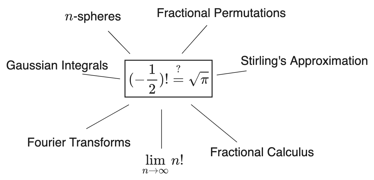
There’s not a well-defined question here, really; it’s just trying to get to the bottom of something. The best way to describe it concisely would be:

Why, morally, does \((-\frac{1}{2})!\) equal \(\sqrt{\pi}\)?

(Always with the caveat that is does not, necessarily: \(\Gamma(x)\) is the best interpolation of \(x!\) to non-integers, but it’s not the only one, since any function which is zero on \(\bb{N}\) can be multiplied by it, giving a “pseudogamma function”.)

We know why it holds algebraically, but otherwise it remains a mostly mysterious fact—connected to lots of things but not exactly “explained” by any of them. If we can find an answer, maybe it will shed light on all the places that \(\pi\) and \(\Gamma\) show up. Or maybe not! Who knows.

Why care about any of this? Well, just for fun, mostly. It’s mostly about recording the chains of thought for posterity. This kind of inquiry tends to seem completely self-explanatory to some people and absurd to others. Personally I just enjoy it; it feels more “significant” to search for the philosophical meaning of a thing than to look for a new identity or proof or something like that. And who knows, maybe we’ll discover something useful along the way.

---

1. The Story So Far

In Investigations on n-Spheres I came to the rather-appealing form of the formula for the volume of an \(n=2k\)-sphere,

\[V_{2k} = \frac{(\pi r^2)^k}{k!}\]

This is just a rephrasing of the usual formula, but is a bit more compelling (and easier to remember). It’s exactly the same form as the volume of a tetrahedron (/ \(k\)-simplex) with side-length \(a = \pi r^2\), yet is also valid at half-integer \(k\).

Perhaps this suggests something about how to interpret the haf-integer factorials as permutations of sets with half-integer numbers of elements? Hopefully!—because that seems like the only way to say anything concrete about any of this. The only satisfying answer is to find some sort of “geometric” model of what’s going on. Otherwise it is hard to argue that \(\Gamma\) is even the “correct” interpolation of \((n!)\). The fact that \(\Gamma\) is the unique function that obeys certain properties isn’t a good-enough reason: every function is the unique function that obeys a certain property, namely the property of being itself. And anyway, if you define it uniquely in terms of those properties then you have only rephrased the question: you still need to say what makes those properties special.

No, the thing that makes \(\Gamma\) special is that Nature seems to agree that it is: she has it showing up all over the place, in settings which have nothing obviously to do with either permutations or circles. There is something intrinsic about it and we’d like to say what.

In Factorials as Multiplicative Integrals we discussed how the double-factorial’s asymptotic behavior is different between even and odd factorials, and the discrepancy is entirely due to the fact that, when written as an multiplicative integral, it is over a slightly different integration range:

\[n!! \equiv \begin{cases} \prod_0^n d^{\times}(n!!) & n \text{ even} \\[1em] \prod_1^n d^{\times}(n!!) & n \text{ odd} \\ \end{cases}\]

In particular the missing piece of the odd double factorial corresponds to the value of \(\sqrt{\pi}\).

\[\prod_0^1 d^{\times}(n!!) = \sqrt{2} \prod_0^{1/2} d^{\times}(n!) = \sqrt{2} (\frac{1}{2})!= \sqrt{\frac{\pi}{2}}\]

Again this is (somewhat) numerology; nothing about the factorial function so far really necessitates writing it as an integral or justifies thinking of it as continuously interpolated in an unambiguous way. That said, there is a fairly-concrete interpretation of the fractional factorial as being defined by asymptotic ratios of integer factorials, for instance

\[\begin{aligned} (-\frac{1}{2})! &\approx \frac{(2k+1)!!}{2^k (k+1/2)!} \\ &= \lim_{k \ra \infty} \frac{(2k+1)!!}{2^k k! \sqrt{k}} \end{aligned}\]

This is essentially equivalent to the previous point, since as just mentioned the value of \((2k+1)!!\) is proportional to \(\sqrt{\pi}\) precisely because of how it omits the value of \((-1/2)!\). But, since this version is defined entirely on integers, it is credible as a “definition” of \((-1/2)!\).

The arguments for these sorts of identities all run circles (…) around each other; most of them involve, in one way or the other, either Stirling’s approximation

\[n! \sim \sqrt{2 \pi} (\frac{n}{e})^n\]

And/or the Wallis Product

\[\frac{\pi}{2} = \sum_n \frac{(2n)!! (2n)!!}{(2n-1)!!(2n+1)!!}\]

Each of which can be derived from the other.

Despite all these connections it’s hard to say what “causes” what, even if you’re willing (as I am) to think of one notion in math as “causing” another. Is \((-1/2)! = \sqrt{\pi}\) “due to” Stirling’s approximation? Or the other way around? And why do these end up having to do with the volumes of spheres?

One satisfying approach to claiming that an identity \(A\) should be said to “cause” another identity \(B\) (despite each being equivalent) is that there is a natural framework in which to generalize \(A\), such that \(B\) falls out as a special case in a larger family of identities. In particular we expect that if two identities imply each other then under the hood there is some “geometric” structure (abstractly speaking) that each formulation is describing. It’s the geometry that is the intrinsic thing; the equations are just snapshots of it from different angles. Once we find that geometry, we go looking for the larger class that it is a member of, and those siblings will provide other equations that generalize \(A\).

That’s the idea, at least.

For \(\Gamma\) specifically, we have to assume that any equation that produces a factor of \(\pi\) exhibits some kind of circular symmetry, somewhere. The fact that this is hard to see in the case of \((-\frac{1}{2})! = \Gamma(\frac{1}{2}) = \sqrt{\pi}\) is precisely why I’ve been so distracted by investigating this. Where is the intrinsic circular symmetry here? What do its asymptotics, interpolations, etc have to do with spherees? And let’s not forget that \(\pi\) itself is somewhat “arbitrary”. Is there some even-more-fundamental thing going on here, maybe connected to permutations, that “causes” \(\pi\) to have the value that it has?

Well, in the remainder of this article I will discuss some of the connections between \((-\frac{1}{2})! = \sqrt{\pi}\) and circular symmetry. But none of them shed more light on what’s going on: they’re basically restatements of the same identities we’ve already found. Nevertheless I wanted to make a record of them, for completeness and so I can refer to the later (and, of course, because they’re neat—these tend to be arguments that most people will not have seen before, yet are not too hard to follow with a standard background in math or physics).

---

2. Gaussian Integrals

Many of the places you see \(\sqrt{\pi}\) around math and physics involve Gaussian integrals:

\[I = \int_{-\infty}^{\infty} e^{-x^2} \d x\]

Most people who have studied math will have come across the standard trick for evaluating \(I\): square it as two separate integrals, combine the two linear integration variables into one integrand, and then change variables to \((r, \theta)\):

\[\begin{aligned} I^2 &= [\int_{-\infty}^{\infty} e^{-x^2} \d x] [\int_{-\infty}^{\infty} e^{-y^2} \d y] \\ &= \int_{\bb{R}^2} e^{-(x^2 + y^2)} \d x \d y \\ &= \int_0^\infty \int_0^{2 \pi} e^{-r^2} r \d r \d \theta \\ &= 2 \pi (-\frac{1}{2} e^{-r^2} \big|_0^{\infty}) \\ &= \pi \\ \end{aligned}\]

Giving \(I = \sqrt{\pi}\).

Somewhat less known is that you can compute this integral by raising \(I\) to whatever power you want. Regardless of the power, the substitution \(z = r^2\) turns the integral into a Gamma function—and then the coefficient that comes out is the volume of the \(n\)-sphere, instead of the \(2\)-sphere. Tthis can be seen as a way of computing \(S_n\) in the first place:

\[\begin{aligned} I^n &= \int_{\bb{R}^n} e^{-(x_1^2 + x_2^2 + \ldots x_n^2)} \d^n x \\ &= \int_0^{\infty} \int_{S^{n-1}(r)} e^{-r^2} r^{n-1} \d r \d S^{n-1} \\ &= S_{n-1}(1) \int_0^{\infty} e^{-r^2} r^{n-1} \d r \\ &= S_{n-1}(1) \frac{1}{2} \int_0^{\infty} e^{-z} z^{n/2 - 1} \d z \\ (\sqrt{\pi})^n &= S_{n-1}(1) \frac{1}{2} \Gamma(\frac{n}{2}) \\ S_{n-1}(1) &= \frac{\pi^{n/2}}{\frac{1}{2}\Gamma(\frac{n}{2})} = \frac{n \pi^{n/2}}{(\frac{n}{2})!} \end{aligned}\]

Which is pretty cute, in my opinion. The \(I^2\) case is actually the \(n=1\) case of this, because a \(0\)-sphere is two points and the “surface area” is \(S_0(1) = 2\):

\[I = \int_{-\infty}^{\infty} e^{-x^2} \d x = 2 \int_0^\infty e^{-x^2} \d x = S_0(1) \frac{1}{2} \Gamma(\frac{1}{2})\]

Also cute. But weird too, right? It feels like it’s hiding something important. What’s going on here when we multiply products of \(1\)-spheres to make \(n\)-spheres? Well, there are a few things to unpack here, so let’s poke around.

It’s generally the case that you can factor a spherically-symmetric integral in this way. If \(f(x_1, x_2, \ldots) = f(r)\), then an integral of \(f(r)\) can be factored by Stokes’ theorem into radial and angular terms, via

\[\begin{aligned} \int_{\bb{R}^n} f(x_1, x_2, \ldots) &= \int_{\bb{R}^n} f(r) \d V \\ &= \int_{0}^{\infty} \int_{\p V_n(r)} f(r) d (\p_r V_n(r)) \d r \\ &= \int_0^{\infty} \int_{S_{n-1}(r)} f(r) S_{n-1}(r) \d r \\ &= S_{n-1}(1) \int_0^{\infty} f(r) r^{n-1} \d r \end{aligned}\]

It’s somewhat clear why Gaussian integrals involve the factors of \(S_n\): the product \(I^n\) has \(n\)-spherical symmetry, because once you have \(e^{-(x_1^2 + x_2^2 + \ldots)}\) as the only term inside the integral, it is unchanged by rotations on the surface of the \(n\)-sphere. I suppose it is a general rule that if an integral has a symmetry, the “volume” of that symmetry group shows up as a coefficient in the result, because you can integrate it out first. So \(S_{n-1}\) shows up in the result, and since each product of another \(I\) increases the dimension of the sphere, the Gaussian products must obey the same recurrence relations as the \(n\)-sphere areas.¹

You won’t find the same pattern in any other integrals: the property that \(I[x^2] I[y^2] = I[x^2 + y^2]\) only works with exponentials. But perhaps an analogous idea might work somewhere else. I would not be surprised to learn that there are equivalent identities for shapes other than \(n\)-spheres. What kind of integrand is invariant under displacements on the Lemniscate such that its value is proportional to \(\varpi\), the lemniscate constant, I wonder? I have no idea. But probably one exists (presumably \(e^{-x^4}\)?), and probably it has something to do with \(\Gamma(1/4) = \sqrt{2 \varpi \sqrt{2 \pi}}\).

So I am fine with Gaussians being proportional to \(\sqrt{\pi}\), because their square is proportional to \(\pi\). And it certainly seems to suggest something about the meaning of \(\Gamma(\frac{1}{2}) = (-\frac{1}{2})! = \sqrt{\pi}\). But I can’t quite tell what it is. We know that the Gaussian integral value is “caused” by the \(n\)-sphere, in the sense that it’s due to the spherical symmetry of the integral, and that the Gaussian integral is transformable into \(\Gamma\). Do things go the other way? Do the half-integer factorials get their values because of the \(n\)-spheres? Does \(S_0 = \frac{2 \pi^{1/2}}{(-\frac{1}{2})!} = 2\) “cause” \((-\frac{1}{2})! = \sqrt{\pi}\)? Probably not; they’re just equivalent. What we need is some kind of connection with the combinatoric interpretation of factorials that explains both of these.

Another curious observation: since \(\int_{-\infty}^{\infty} e^{-x^2} \d x = \sqrt{\pi}\), a change of variables \(x = \sqrt{\pi} r\) gives the suggestive-looking

\[\int_{-\infty}^{\infty} e^{-\pi r^2} \d r = 1\]

Where the exponent is clearly \(V_2(r) = \pi r^2\). I think this is significant. Whatever was going on with \(V_{2k} = (\pi r^2)^k/k!\) which has the right form in the variable \(x = \pi r^2\) is clearly being demonstrated here also. Probably the two are just restatements of each other. But how do we make sense of it? I don’t know at the moment, but we will surely be coming back to this.

---

3. Fourier Transforms

Now a slight change of subject. Recall that in all the definitions of the Fourier transform there is a factor of \(1/2\pi\) that you pick up somewhere between the transform and its inverse:

\[\begin{aligned} \F[f(x)](k) &= \int_{-\infty}^{\infty} f(x) e^{-ikx} \d x \\ \F^{-1}[\hat{f}(k)](x) &= \frac{1}{2 \pi}\int_{-\infty}^{\infty} \hat{f}(k) e^{ikx} \d x \\ \end{aligned}\]

Of course there are many slightly-different definitions of Fourier transforms on differently angles (see them all here)—but there’s always either a factor of \(1/2\pi\) on one or the other, or a \(1/\sqrt{2\pi}\) on each, or something like that. This factor is definitely related to the Gaussian and \((-\frac{1}{2})!\) and everything else we’re looking at, so let’s study it a bit.

One way to think about that factor is that it is required because the inverse transform is almost like applying \(F\) again, but not quite, because \(\F^2\) is not \(I\) exactly. It has an extra factor and the wrong sign:

\[\begin{aligned} \F^2[f(x)] &= \F[\hat{f}(k)](x) \\ &= \int_{x=-\infty}^{\infty} \hat{f}(k) e^{-ikx} \d x \\ &= 2 \pi \big[ \frac{1}{2\pi} \underbrace{\int_{x=-\infty}^{\infty} \hat{f}(x) e^{i(-k)x} \d x}_{\text{swap } k \lra x} \big] \\ &= 2 \pi \F^{-1}(\hat{f}(-x)) \\ \end{aligned}\]

So \(\F[f](x)\) is almost its own inverse, and \(f \mapsto \frac{1}{2 \pi} \F[f](-x)\) actually is. Since \(\F^2[f] = \frac{1}{2\pi}f(-x)\), you will see the Fourier transform described as a rotation in \((x,k)\) space. This is apparently not quite true: evidently the integral itself is proportional to a rotation times a factor of \(\sqrt{2 \pi}\), such that \(\F^2 = -2 \pi I\) instead of \(-I\).

Suppose we didn’t know what the value of the \(2\pi\) factor was; how do we find out? Well, it turns out that we can derive its value from Gaussian integral, suggesting they are also expressing the same idea. The argument goes: consider \(\F^2[f(x)] = 2 \pi f(-x)\), but suppose we didn’t know the constant yet.²

\[\F^2[f(x)] \? K f(-x)\]

We will figure it out like this:

Fourier transforms of functions that go to zero at infinity have the property that they interchange coordinates and derivatives: \(\F[f'(x)] = ik \F[f(x)]\) and \(\F[x f] = i \p_k \F[f]\). This can be seen by messing around with the form of \(\F\) and doing some integration-by-parts:

\[\begin{aligned} \F[f'(x)] &= \int f'(x) e^{-ikx} \d x \\ &= f(x) e^{-ikx} \big\|_{-\infty}^{\infty} - \int f(x) \p_x e^{-ikx} \d x \\ &= (ik) \F[f(x)] \\[1em] \F[x f(x)] &= \int x f(x) e^{-ikx} \d x \\ &= (i \p_k) \int f(x) e^{-ikx} \d x \\ &= (i \p_k) \F[f] \end{aligned}\]

A Gaussian \(G(x) = e^{-x^2/2}\) (note the new factor of two in the exponent compared to the integrals in the previous section) obeys the differential equation \(\p_x G = -x G\) . Since the Fourier transform swaps the derivative and coordinate, \(\F[G]\) produces the same differential equation again, and therefore \(\hat{G}\) is another Gaussian (this is one way of thinking about why the Fourier transform of a Gaussian is another Gaussian):

\[\begin{aligned} \F[\p_x G(x)] &= \F[- x G(x)] \\ &\Ra \\ ik \F[G] &= -i \p_k \F[G] \\ k \hat{G} &= - \p_k \hat{G} \end{aligned}\]

The solution to this differential equation is another Gaussian \(\hat{G}(k) = C e^{-k^2/2}\), with \(C\) an integration constant:

\[k [C e^{-k^2/2}] = -\p_k [C e^{-k^2/2}]\]

To find the value of \(C\), we evaluate \(\hat{G}(0) = \F[G](0)\), which becomes the standard Gaussian integral:

\[\begin{aligned} \F[G](k) &= \int_{-\infty}^{\infty} e^{-x^2/2} e^{-ikx} \d x \\ \F[G](0) &= \int_{-\infty}^{\infty} e^{-x^2/2} \d x \\ &= \int_{-\infty}^{\infty} e^{-y^2} \d (\sqrt{2}y) \\ &= \sqrt{2\pi} \end{aligned}\]

Meanwhile squaring the Fourier transform and using the fact that \(G(x) = G(-x)\) tells us what the coefficient \(\F^2[f] = K f(-x)\) has to be:

\[\begin{aligned} \F^2[G] &= \F[\sqrt{2 \pi} e^{-k^2/2}] \\ K G(-x) &= 2 \pi G(x) \\ K &= 2 \pi \end{aligned}\]

In summary, the Gaussian \(G = e^{-x^2/2}\) is the function which has \((x + \p_x) G = 0\). The definition is invariant under \(x \lra \p_x\), which is what \(\F\) does, hence it is unchanged by Fourier “rotations”. Since \(\F[G](0) = \sqrt{2 \pi}\), though, the rotations must accumulate that factor, which is why we have to divide it off in the inverse transform.

So, the Gaussian integral \(\lra\) Gamma function \(\lra\) \(n\)-sphere correspondence also extends to the Fourier transform definition. Not too surprising, but at least it maybe takes Fourier transforms off the table for telling us anything new: they’re just the same idea in a different form.

---

4. Stirling’s Approximation

Earlier we discussed the fact that one definition of \((-1/2)!\) gives it as being “induced” by the asymptotic behavior of \(n!\). I’ll repeat the argument, which I came across in this form in this post, here.

There’s a good reason to expect that, as \(n \ra \infty\),

\[(n+1/2)! \sim (n)! \sqrt{n}\]

Since \((n+1)! = (n+1) \times n!\), it should take roughly two factors of order \(\sqrt{n+1} \approx \sqrt{n}\) to get from \(n!\) to \((n+1)!\), and by the same logic, roughly one factor of order \(\sqrt{n}\) to get from \(n!\) to \((n+1/2)!\).

Given that, we can then write out each term as an actual factorial, producing an identity for \((1/2)!\):

\[\lim_{n \ra \infty} \frac{(n+1/2)!}{(n)! \sqrt{n}} = \lim_{n \ra \infty} \frac{(n + \frac{1}{2}) \times (n - \frac{1}{2}) \times \ldots \times \frac{3}{2} \times (\frac{1}{2})!}{n \times (n-1) \times \ldots \times 2 \times 1 \times \sqrt{n}} = 1\]

And so, flipping this around, this could be regarded as the justification for the value of \((\frac{1}{2})!\):

\[\begin{aligned} (\frac{1}{2})! &= \lim_{n \ra \infty} \frac{n \times (n-1) \times \ldots \times 2 \times 1 }{(n + \frac{1}{2}) \times (n - \frac{1}{2}) \times \ldots \times \frac{5}{2} \times \frac{3}{2}} \times \sqrt{n} \\ &= \lim_{n \ra \infty} \frac{n! \sqrt{n}}{ 2^{-n}(2n+1)!! } \\ &= \lim_{n \ra \infty} \frac{(2n)!! \sqrt{n}}{(2n+1)!!} \\ \end{aligned}\]

Which works out to be \(\sqrt{\pi}/2\). I suppose repeating this with \((n+1/3)!\) or anything else would provide a justification for the corresponding values of \((\frac{1}{3})!\), etc: although it won’t give an analytic expression, it would justify why it has that particular decimal value. Note that this is a first-order approximation; the Wallis Product gives an exact version (presumably because in the limit all the errors cancel each other out).

While this argument works, I don’t think it’s a great justification for the source of the \(\sqrt{\pi}\). Really it just reflects the fact that that the mysterious \(\sqrt{\pi}\) factor continues to be present in the half-integer factorials off to infinity, without giving a reason why. And it kicks the question over to why Stirling’s Approximation

\[n! \sim \sqrt{2 \pi n} (\frac{n}{e})^n\]

holds, since that is more-or-less the source of the asymptotic behavior.

The \(\sqrt{\pi}\) in Stirling’s formula can be derived from the Wallis Product as well, but there is an argument to be made that it is somewhat more fundamental than that. In fact it comes more directly from the Gaussian integral: it’s a factor that shows up in any integral of the form \(\int e^{M f(x)} \d x\) as \(M \ra \infty\), given a few requirements (if it has a maximum \(f(x_0)\) which inside the integration range, plus some differentiability conditions). That’s because as \(M \ra \infty\) the dominant term in the integral can be factored out as a Gaussian integral, a technique known as Laplace’s Method:

\[\begin{aligned} \lim_{M \ra \infty} \int e^{M f(x)} \d x &= \lim_{M \ra \infty} e^{M f(x_0)} \int e^{-\frac{1}{2} M f''(x_0) (x-x_0)^2} \d x \\ &= \sqrt{\frac{2 \pi}{M \| f''(x_0) \|}} e^{M f(x_0)} \end{aligned}\]

Which again produces a \(\sqrt{\pi}\) term. Although the technique is just that, a technique, the “presence” of the Gaussian is there either way: it reflects an underlying property of the function \(f(x)\). As such integrals of the form \(\int e^{M f(x)} \d x\) will generally have a Gaussian factor. This includes \(n!\), which can be written

\[n! = \int_0^{\infty} x^n e^{-x} \d x = e^{n \ln n} n \int_0^{\infty} e^{n(\ln y - y)} \d y\]

This obeys the conditions for Laplace’s method, therefore it has a Gaussian-like second-order term that dominates its \(M \ra \infty\) limit and makes the first term in its asymptotic expansion \(\propto \sqrt{\pi}\).

After that, the same argument for the \(\sqrt{\pi}\) in Gaussians kinda shows up here again: square this integral and you get something circularly symmetric to second-order. Etc. So we might deduce that the ‘causality’ is: the factorial picks up a factor of \(\sqrt{\pi}\) in its asymptotics (which is reflected in its half-integer values…) because it acts like the integral of an exponential \(e^{n \ln y - ny}\). Not particularly illuminating, but not nothing, either.

So \(n\)-spheres cause Gaussians which cause \(\sqrt{\pi}\) which causes factorials to show up in \(n\)-spheres again? Everything seems to be going in… circles.

---

5. Fractional Calculus

Fractional Calculus is what you get when you try to generalize the familiar formulas of calculus

\[\begin{aligned} D_x^k \frac{x^n}{n!} &= \frac{x^{n-k}}{(n-k)!} \\[1em] D_x^k e^{ax} &= a^{k} e^{ax} \\[1em] \underbrace{\int_0^x \big( \int_0^{x_1} (\ldots f(x) \ldots) \d x_2 \big) \d x_1}_{n \text{ times}} &= \frac{1}{(n-1)!} \int_0^x (x-t)^{n-1} f(x) \d t \\ \F[x^n f(x)] &= (i D_k)^n \F[f(x)] \\ \end{aligned}\]

to non-integers in the obvious ways. For example presumably \(D^k\) ought to obey \(D^{a} D^{b} = D^{a+b}\) whether or not the exponents are integers, and therefore \(D^{1/2} D^{1/2} = 1\) and \(D^a \int_0^x f(x') dx' = D^{a-1} f\).

Unfortunately, nothing is simple: if you take each of those equations as you starting point you get a different, non-equivalent generalization of integer calculus. Take a look at all the different definitions on the wiki. I think it is safe to say that this subfield of math is a mess that needs cleaning up. How would you know which of these to use if you came upon some differential equation in physics? You wouldn’t, is how. But apparently it does find its uses.

One issue is that the resulting formula are pretty bizarre. What is to be made of expressions like (using the first generalization above)

\[\begin{aligned} D^{1/2} x &\? \frac{x^{1/2}}{(\frac{1}{2})!} = \frac{\sqrt{x}}{\sqrt{\pi}/2} \\ \end{aligned}\]

Or (using the second), should this be multivalued across a bunch of roots of unity or something?

\[D^{1/k} e^{ax} = \sqrt[k]{a} e^{ax}\]

Another thing that defies simple explanation is that a fractional derivative is inherently nonlocal. Whereas a discrete derivative only involves points in the immediate vicinity of where you compute it,

\[D_x f(x) = \lim_{dx \ra 0} \frac{f(x + dx) - f(x)}{dx}\]

the fractional derivative ends up involving something like an integral over the whole domain of the function: an infinite sum of \(f(x + n \d x)\) for \(n \in \bb{N}\). The simplest way of seeing this is to consider a discretized version of derivative:

\[D_x f(x) \approx \frac{(T_{dx} - I)}{dx}\]

And so the nested derivative looks like raising this to a power:

\[\begin{aligned} D^n_x &= (\frac{(T_{dx} - I)}{dx})^n \\ &= \frac{1}{dx^n} [(T_{dx} - I)(T_{dx} - I)(T_{dx} - I) \ldots] \\ &= \frac{1}{dx^n} [T_{dx}^n - \binom{n}{1} T_{dx}^{n-1} + \binom{n}{2} T_{dx}^{n-2} \ldots \pm n T_{dx} \mp I] \end{aligned}\]

Where \(T_{dx}^k f(x) = T_{k \d x } f(x) = f(x + k \d x)\). For integer \(k\) every term is near where you started, and so in the limit \(dx \ra 0\) they become an infinitesimal measure of the change in \(f(x)\). But one fractional derivative comes by just replacing \(k\) with a non-integer and then using the (!!) non-integer binomial expansion, which has infinitely many terms:

\[D^n_x = \frac{1}{dx^n} ( \sum_{k = 0}^{\infty} \binom{n}{k} T_{dx}^k (-I)^{n-k})\]

This is immediately hard to interpret, because \((-1)^{n-k}\) is a non-integer power and so is normally thought of as multivalued and is forced to be imaginary for odd \(n-k\), and what is that supposed to mean? So, okay, there’s a trick you can use: maybe you generalize from the “backwards” derivative

\[D_{x} f(x) = \frac{(I - T_{-dx})}{dx}\]

instead, giving

\[\begin{aligned} D^n_x &= \frac{1}{dx^n} [\sum_{k = 0}^{\infty} \binom{n}{k} I^k (-T_{-dx}^{n-k} )] \\ &=\frac{1}{dx^n} (1 - \binom{n}{1} T_{-dx} + \binom{n}{2} T_{-dx}^2 + \binom{n}{3} T_{-dx}^3 - \ldots) \end{aligned}\]

and then you have one fewer problems because the non-integer powers of \((-1)\) are hiding out at the infinite end of the series… but you’re still in trouble. What is the meaning of the binomial expansion for non-integer values anyway? Well, apparently lots of the algebra of combinatorics continues to work when you let the factorials become Gamma functions:

\[\binom{1/2}{1} = \frac{(\frac{1}{2})!}{(1)! (\frac{1}{2}-1)!} = \frac{\frac{\sqrt{\pi}}{2}}{\sqrt{\pi}} = \frac{1}{2}\]

For example, fractional binominal expansions end up giving perfectly-legitimate Taylor series:

\[(1 + x)^{1/2} = 1 +\frac{1}{2} x - \frac{1}{8} x^2 + \frac{1}{16} x^3 + \ldots\]

Which converges if \(\| x \| < 1\). (Disconcertingly, you can also expand the sum into negative powers instead of positive ones, \(\sum_{k=-\infty}^{-1} \binom{1/2}{k} x^k\), which gives a Taylor series for the same function but around \(x=\infty\) instead of \(x=0\).) And generally the generalized binomial coefficients on non-positive-integers obey almost all of the same algebraic identities as the usual ones. So there’s definitely something going on there.

The same thing can be used to create fractional derivatives:

\[\begin{aligned} D^{1/2}_x &= \frac{1}{\sqrt{dx}} (I - T_{dx})^{1/2} \\[1em] &= \frac{1}{\sqrt{dx}} (I + \frac{1}{2} T_{-dx} - \frac{1}{8} T_{-2 dx} + \frac{1}{16} T_{-3 dx}\ldots) \\ \end{aligned}\]

Which basically amounts to an integral: if you imagine taking the limit \(dx \ra 0\) while extending the sum to \(N \ra \infty\) terms such that \(N \d x = a\) is fixed, then it’s a sum of values of \(f\) at every \(f(x - k \d x)\) between \(x\) and \(x-a\), that is, something kinda like

\[D^{1/2}_x f(x) \sim \int_{x}^{x-a} f(x') \underbrace{\frac{1}{\sqrt{dx'}}}_{\text{??}}\]

Whatever that means. (It’s definitely not correct as-written; I’m just making up a notation there.)

So the fractional derivative is a nonlocal operation, more like an integral than a derivative. Not only that, but we seem to have some freedom over which integral it is depending how we take the limits? This is the source of some of the variation in definitions of fractional derivatives (see here) but not all of it. (Incidentally, this is the same problem you get when trying to define an integral as an “inverse derivative operator”: clearly \(D_x^{-1} f(x) \? \int f(x) \d x\) needs to get its integration bounds from somewhere, but where?)

Regardless of how you solve all of this, it’s clear that fractional calculus is very closely connected to “fractional combinatorics”, which means that to assign meaning to it we really do need to be able to say what’s going on with \((1 + x)^{1/2}\) as well. And a satisfying answer for that is necessarily going to involve contending with interpolating permutations between integers, and possibly some sense of “fractional sets”. I have no doubt that that’s where we’re going, as it seems like the heart of the thing… but it’s too early for that. This article is just about staring at the walls from different directions and looking for cracks.

Incidentally, plenty of people have sought geometric interpretations for fractional derivatives (see e.g. here here), but I think most would agree that the best explanations available are still quite sketchy. I’ve skimmed some books and found very little in the way of lucid interpretation. Still, the whole fractional calculus is clearly well-behaved, as numerous examples show: the fractional derivatives and integrals do, for the post part, cleanly interpolate between their integer equivalents.

---

The most digestible reference I have found on fractional calculus is a pdf “Construction & applications of the fractional calculus” by Nicholas Wheeler (whose lucid writing on weird math I have also plugged elsewhere…), which includes numerous examples of applications to non-pathological physical problems. But still Wheeler does not really search for a concrete physical interpretation, probably because it’s a dead end. It just works and that’s all you can say.

However. Wheeler does come right up to (before sadly turning around) what I think is the most important relationship between all these concepts that I’ve seen so far.

I mentioned earlier that the volume of the \(n = 2k\)-sphere is compellingly written in a form that looks like the volume of an \(k\)-simplex with side-length \(\pi r^2\):

\[V_{2k}(r) = \frac{(\pi r^2)^k}{k!} = \frac{a^k}{k!}\]

And this formula does work for half-integer \(k\), which is suspicious. Even more interesting, though, is how the half-derivative with respect to \(a\) cleanly takes you from \(V_{2k}\) to \(V_{2k-1}\):

\[\p_a^{1/2} V_{2k}(a) = \p_a^{1/2} \frac{a^k}{k!} = \frac{a^{k-1/2}}{(k-1/2)!} = V_{2k-1}(a)\]

Which is to say

\[\p^{1/2}_{\pi r^2} \frac{(\pi r^2)^{k}}{k!} = \frac{(\pi r^2)^{k-1/2}}{(k-\frac{1}{2})!}\]

This seems like a strong clue about what’s going on. It’s something like:

“To take the half-derivative of a function \(f(a)\), treat \(a = \pi r^2\) as though it’s the area of a circle in two variables, so \(a^k/k!\) is the volume of a \((2k)\)-sphere… and then reduce the dimension of that sphere by \(1\).”

Still not very cogent, but the source of the \(\sqrt{\pi}\) is in there somewhere. The interpolated derivative is somehow treating the one coordinate \(a\) as an area in two coordinates \(\pi r^2\) such that you can remove “half” a coordinate from it fully-symmetric way. And for some reason, I guess, this requires including that factor of \(\pi\)?

It’s weird. We always had the elementary option of computing \(\p_{\sqrt{x}}\) by rewriting \(x = y^2\):

\[\p_{\sqrt{x}} x^n = \p_y y^{2n} = (2n) y^{2n-1} = (2n) x^{n-1/2}\]

That is, without the \(\pi\) factor. Iterating this gives

\[\begin{aligned} \p^1_{\sqrt{x}} x^n &= (2n) x^{n-1/2} \\ \p^2_{\sqrt{x}} x^n &= (2n)(2n-1) x^{n-1} \\ \p^3_{\sqrt{x}} x^n &= (2n)(2n-1)(2n-2) x^{n-3/2} \\ \p^{k}_{\sqrt{x}} x^n &= \frac{(2n)!!}{(2n - k)!!} x^{n-k/2} \\ \p^{2n}_{\sqrt{x}} x^n &= (2n)!! \end{aligned}\]

Compare to

\[\begin{aligned} \p^{1/2}_x x^n &= \frac{n!}{(n-1/2)!} x^{n-1/2} \\ \p^{2/2}_x x^n &= (n) x^{n-1} \\ \p^{3/2}_x x^n &= \frac{n!}{(n-3/2)!} x^{n-3/2} \\ \p^{k/2}_x x^n &= \frac{n!}{(n-k/2)!} x^{n-k/2} \\ \p^{n}_x x^n &= n! \\ \end{aligned}\]

Somehow this is telling us that the half-derivative is the “better” interpolation. Whereas the \(\p_{\sqrt{x}}\) treats \(x^n\) as being “really” \(y^{2n}\), twice as many elements, the \(\p^{1/2}_{x}\) treats it as really being \(x^n\), \(n\) elements, but locates the “half” permutations in between them. The difference between these is a factor of \(\sqrt{\pi}\) on every other term, and in the end it’s the difference between \((2n)!!\) and \(n!\), as if the reason the \(\p_{\sqrt{x}}\) term doesn’t work is that it’s just “off” by a factor. The factor alternates between \(1/\sqrt{\pi}\) or \(\sqrt{\pi}/2\) on every other element, and after being applied \(n\) times it becomes the ratio \((2n)!!/n! = 2^n\).

Interesting. Seems suggestive? But I don’t see how to make sense of it. I’m lost.

One other thing I will mention is that it very much seems to not be a coincidence that \(\int_{\bb{R}} e^{-x^2} \d x = \sqrt{\pi}\), because it’s really \(\int_{\bb{R}} e^{-\pi r^2} \d r\) that’s equal to \(1\). Whatever this is saying about the interpolation of permutations, it’s showing up in the Gaussian integral also.

More on all this next time as we keep trying to find a way to approach the core of the issue: fractional permutations of fractional sets. And then if that works out, fuck it, maybe we’ll do negatives and imaginary permutations also.

---